library(sp); library(terra); library(gstat)
# unconditional Gaussian simulation on a grid
xy <- expand.grid(1:140, 1:100)
names(xy) <- c("x","y")
gridded(xy) = ~x+y
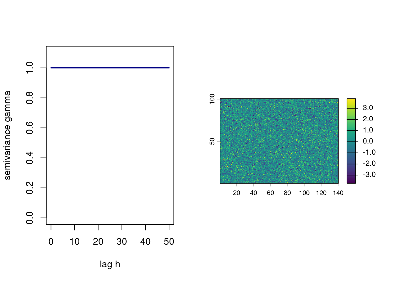
v.m <- vgm(nugget=1, model = 'Sph', psill = 0, range = 0.0001)
plot(variogramLine(v.m, maxdist = 50), type = "l", ylim = c(0,1.1))
g.sim <- gstat(formula = z~1, dummy = TRUE, beta = 0,   model = v.m, nmax = 100)
r.sim <- predict(g.sim, xy, nsim = 1)
plot(rast(r.sim))7 Variograms and their properties
Download slides PDF
The PDF contains what was shown during the lecture. Some of these websites include additional text in light gray.
7.1 Variogram function structure
NoteVariogram
A variogram is a mathematical function that measures how much data points differ from each other based on the distance and direction separating them.
y-axis: semivariance (to measure the similarity of observations)
x-axis: lag (relative distance between points, grouped by bins)
Depending on the form of the variogram function the spatial prediction map will have different properties.
Variogram function is a user choice.
A sample variogram (dots) is plotted from the observed data (dots). A variogram function is fitted to those dots to have a continouous representation (for all distances) of the spatial auto-correlation.
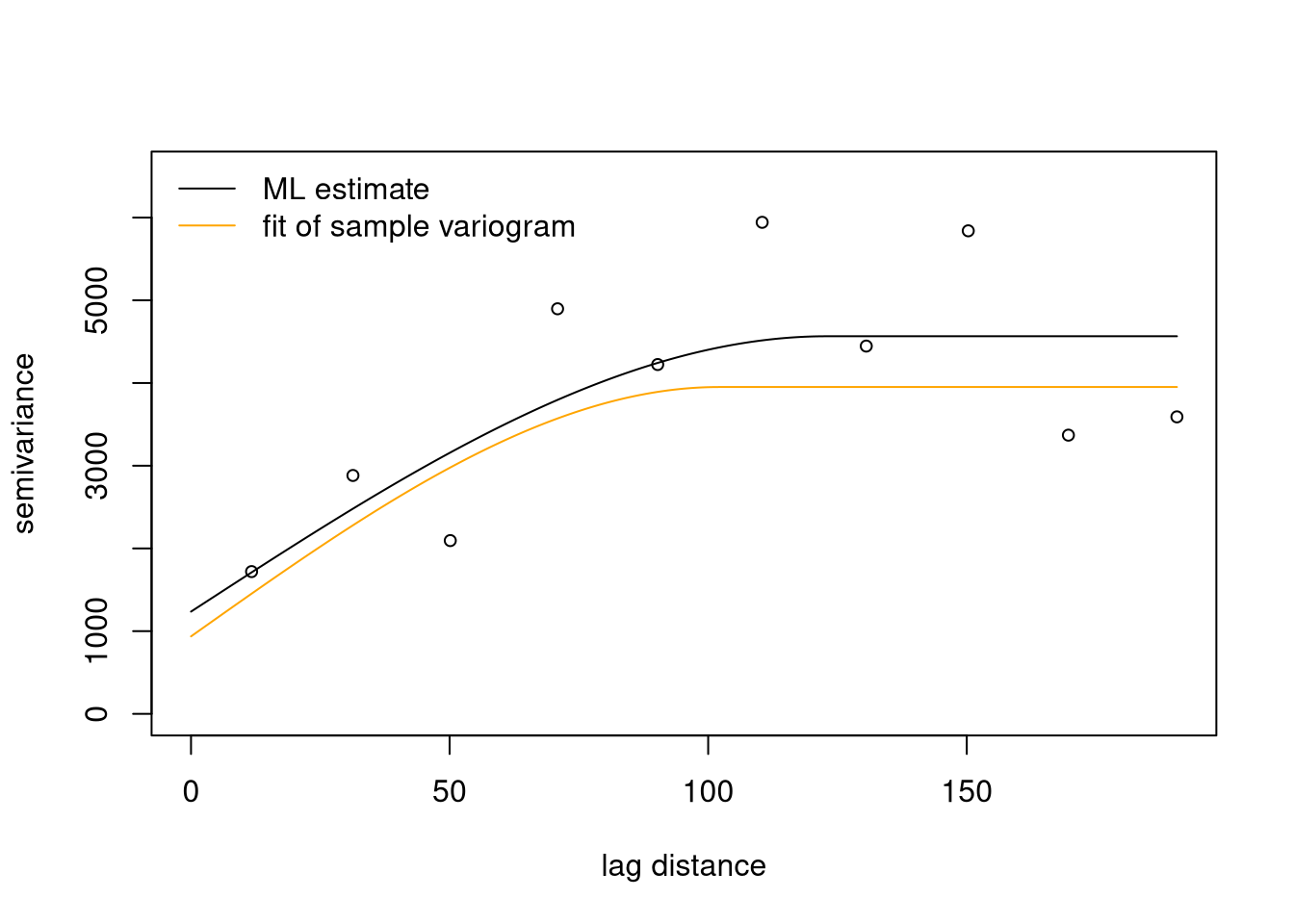
Variogram function structure
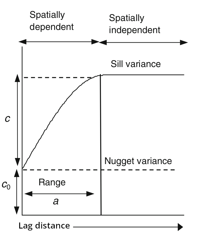
Principle features of the variogram function
Increase in variance with increasing lag
Function must guarantee non-negative variances
Sill variance \(\mathbf{c_0 + c}\), i.e. an upper bound
Range of spatial correlation \(\mathbf{a}\), where auto-correlation becomes 0
Nugget variance \(\mathbf{c_0}\), i.e. a positive intercept or offset to account for smallest scale variability or measurement error
with \(\mathbf{c}\) often called partial sill, i.e. part of variance with spatial structure up to \(\mathbf{a}\)
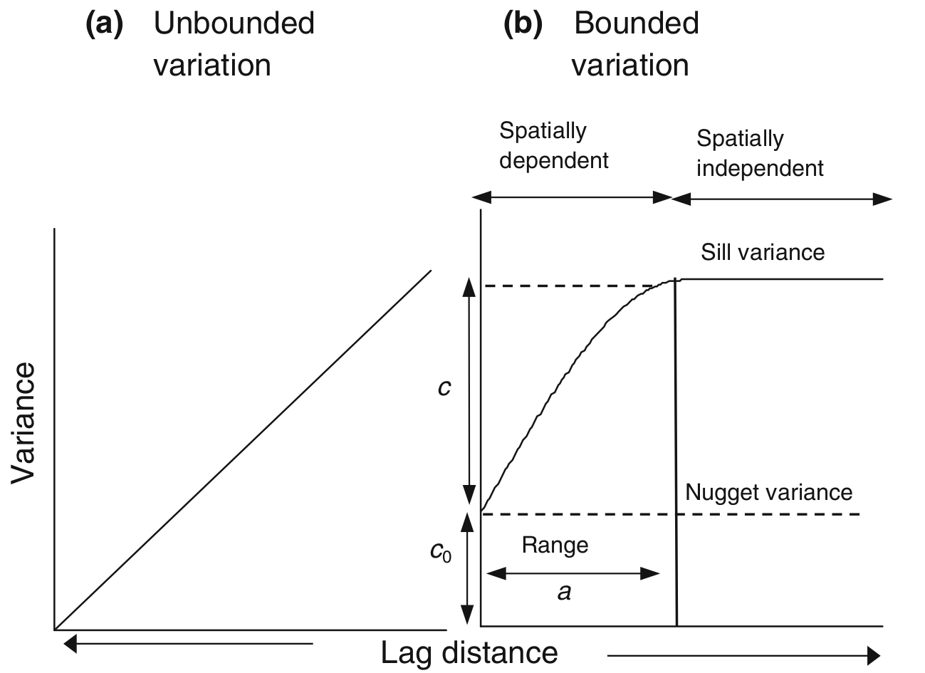
Side note: special cases
Anisotropy, i.e. directional variation depending on angle
Unbounded variogram (not second-order stationary)
Pure Nugget variogram -> no spatial auto-correlation
7.2 Pure nugget variogram
Absence of auto-correlation (nugget effect covariance)
\[ V(h) = \left\{\begin{array}{ll} 0 & \mbox{if $h=0$}\\ c_0 & \mbox{otherwise} \end{array}\right. \]
Mechanism: measurement error and/or small-scale spatial variation
Pure nugget variogram – realization
A realization is a simulation of a random field from the given function.
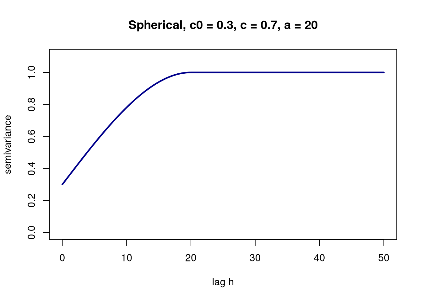
Spherical variogram function
\[ V(h) = \left\{ \begin{array}{lll} c_0 + c \left\lbrace \frac{3h}{2a} - \frac{1}{2} \left(\frac{h}{a}\right)^3 \right\rbrace & \mbox{for $0 < h \leq a$}\\ c_0 + c & \mbox{for $h > a$} \\ c_0 & \mbox{for $h = 0$} \end{array}\right. \]
where \(c_0\) is the nugget variance, \(c\) the variance of spatially correlated component and \(a\) is the range of spatial dependence.
7.3 Spherical variogram function – realizations
A <- vgm(nugget=0.3, model = 'Sph', psill = 0.7, range = 20)
B <- vgm(nugget=0.05, model = 'Sph', psill = 0.95, range = 20)
C <- vgm(nugget=0.3, model = 'Sph', psill = 0.7, range = 5)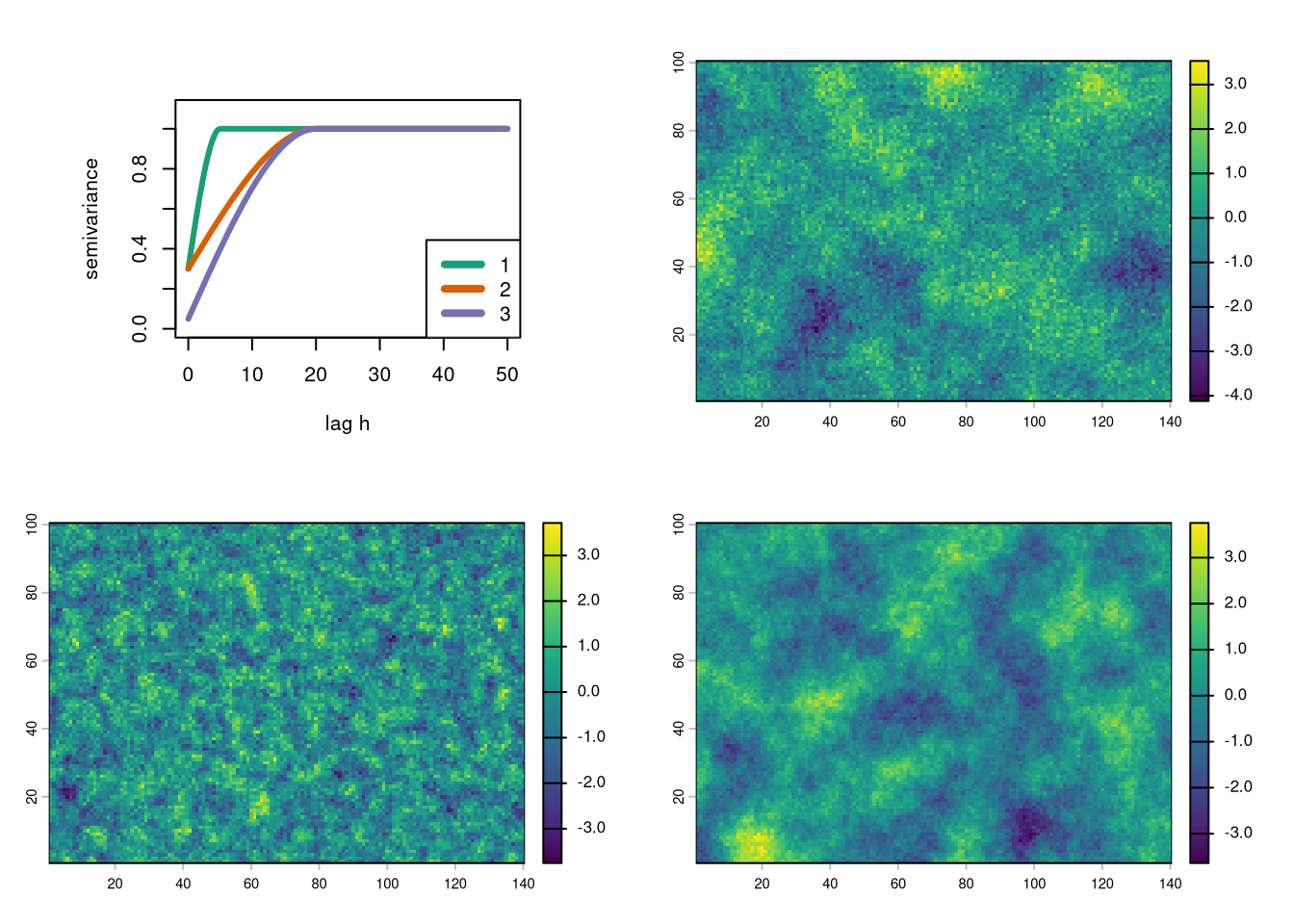
Solution
variogramm model – variogram curve – raster with realization
- A – 2 – top right
- B – 3 – bottom right
- C – 1 – bottom left
7.4 Exponential variogram function
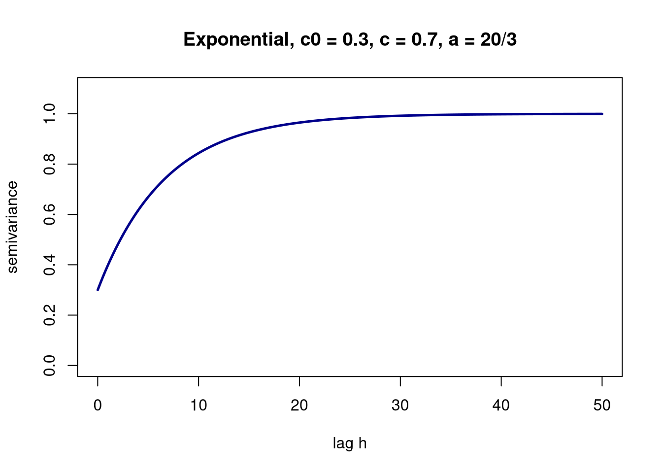
\[ V(h) = \left\{ \begin{array}{ll} c_0 + c \left\lbrace 1 - exp\left(\frac{h}{a}\right) \right\rbrace & \mbox{for $0 < h$}\\ c_0 & \mbox{for $h = 0$} \end{array}\right. \]
with \(a\) here being a distance parameter.
The function approaches the sill asymtotically and does not have a finite range. For practical purposes usually an effective range \(a'\) is used which is approximately \(3a\).
Exponential variogram function – realizations
A <- vgm(nugget=0.3, model = 'Exp', psill = 0.7, range = 7)
B <- vgm(nugget=0.0001, model = 'Exp', psill = 0.999, range = 20)
C <- vgm(nugget=0.1, model = 'Exp', psill = 0.9, range = 20)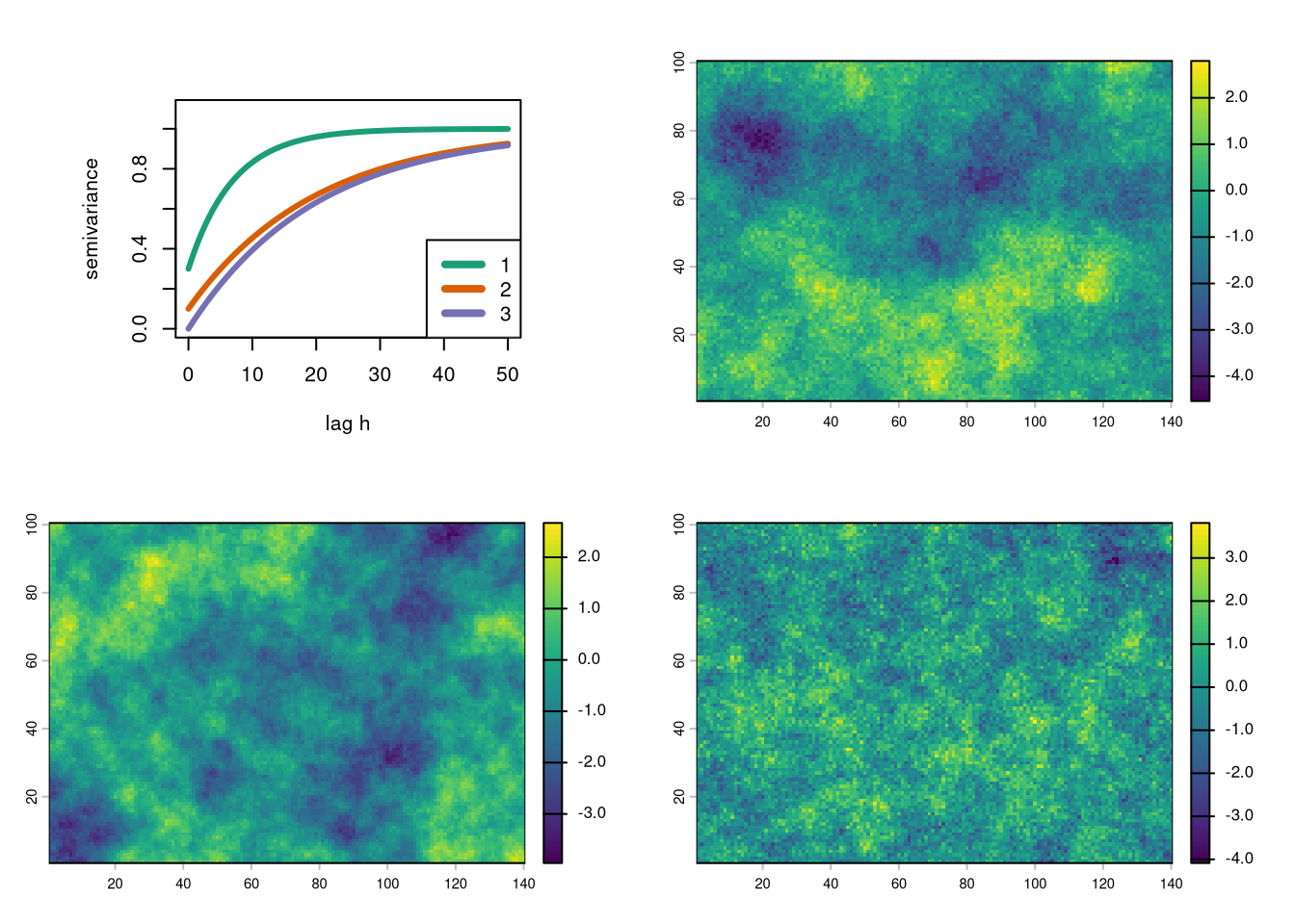
Solution
variogramm model – variogram curve – raster with realization
- A – 1 – bottom right
- B – 3 – bottom left
- C – 2 – top right
7.5 Matérn (Gaussian) variogram function
\[ V(h) = c_0 + c \left\lbrace 1 - \frac{1}{2^{v-1}\Gamma(v)} \left( -\frac{h}{a}\right)^v K_v\left(\frac{h}{a}\right) \right\rbrace \]
with \(c_0\), \(c\) and \(a\) being nugget, sill and range parameters as before.
The equation embodies the gamma function \(\Gamma\) with parameter \(v\) and the Bessel function of the second kind, \(K_v\) for parameter \(v\).
Parameter \(v\) describes the smoothness of variation and can vary from 0 (very rough) to infinity (very smooth).
With \(v=0.5\) it becomes the exponential variogram.
Matérn function – Variogram smoothness
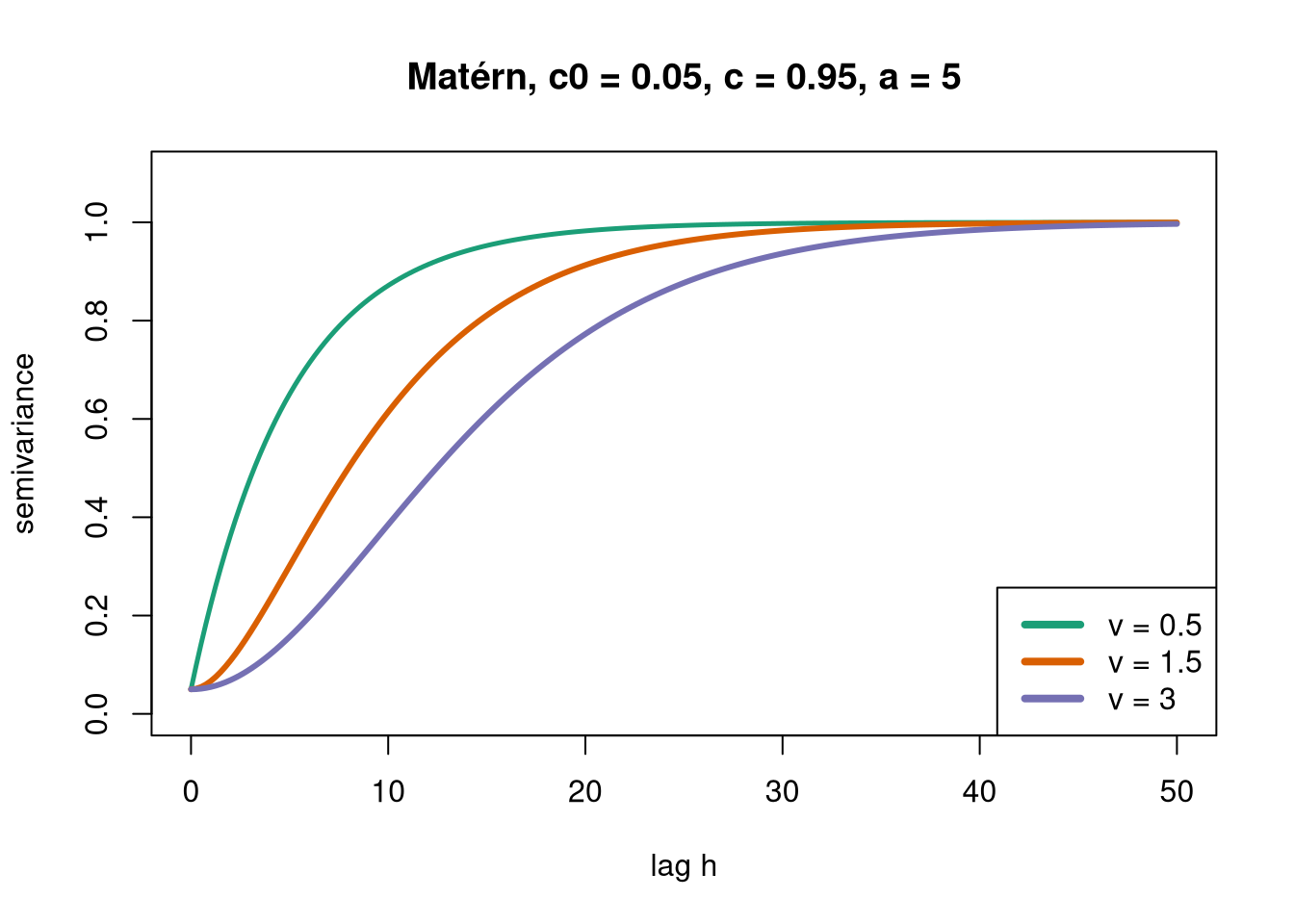
Shape of variogram close to origin controls smoothness of realizations of stochastic processes:
Variogram with nugget: realizations non-continuous
Variogram grows linearly at origin: realizations continuous, but not everywhere differentiable
Variogram grows at at least quadratically at origin: realizations everywhere at least once differentiable
Matérn variogram function – realizations
A <- vgm(nugget=0, model = 'Mat', psill = 1, range = 6, kappa = 0.5)
B <- vgm(nugget=0, model = 'Mat', psill = 1, range = 3.5, kappa = 1.5)
C <- vgm(nugget=0, model = 'Mat', psill = 1, range = 2.5, kappa = 3)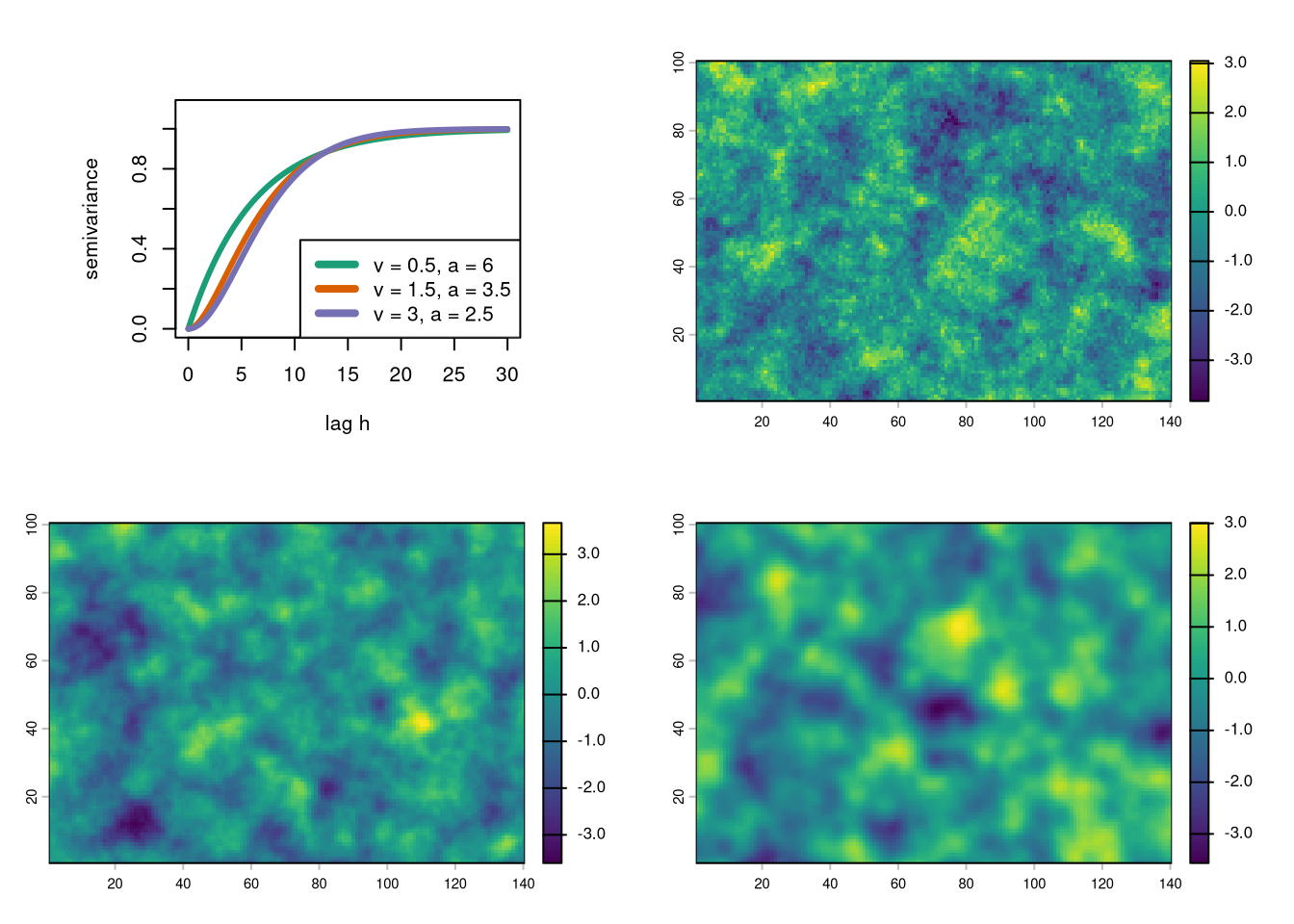
Solution
variogramm model – variogram curve – raster with realization
- A – 1 – top right
- B – 2 – bottom left
- C – 3 – bottom right