library(sf)
library(mapview)
d <- st_read(system.file("shape/nc.shp", package = "sf"), quiet = TRUE)
mapview(d, zcol = "SID79", map.types = "OpenTopoMap")
Number of sudden infant deaths per counties of North Carolina (USA) in 1979.
Download slides PDF
The PDF contains what was shown during the lecture. Some of these websites include additional text in light gray.
e-Lecture video
This lecture is available as recording.
Large number of different sampling designs for various end goals with their estimators.
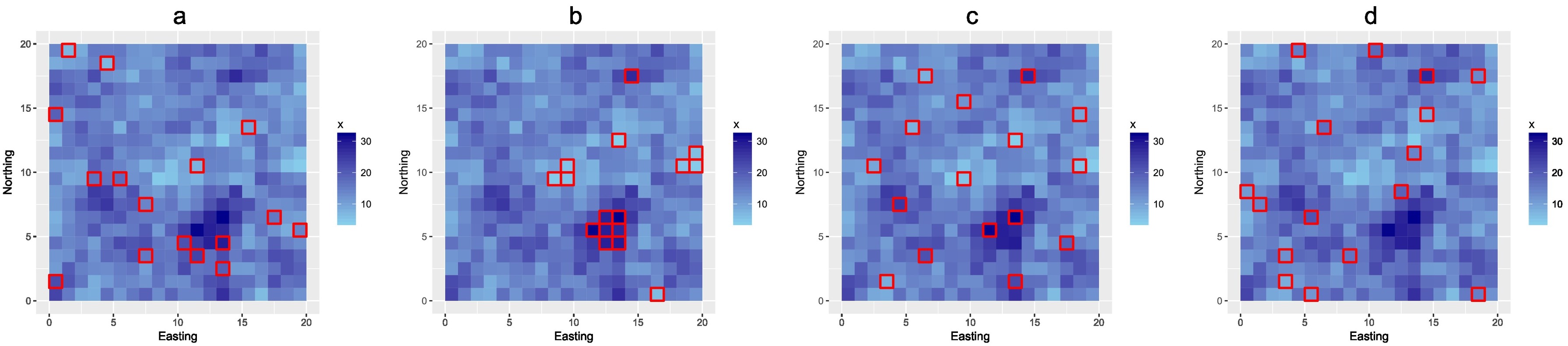
From left to right: simple random sample (a), optimized sample for mapping with linear regression model (b), optimized sample for kriging with an external drift (c), and stratified sample using sixteen equal-sized covariate strata (d). All samples are plotted in a map of the covariate (Brus, 2018).
Brus, D. J. Sampling for Digital Soil Mapping: A Tutorial Supported by R Scripts. Geoderma, 2018.
Brus, D.J. Spatial Sampling with R, 2022, https://dickbrus.github.io/SpatialSamplingwithR
Mean and standard error estimates for finite support targets, e.g. parcels, municipalities.
Example: Soil organic carbon stocks, mapped with robust external-drift kriging for Swiss forests.
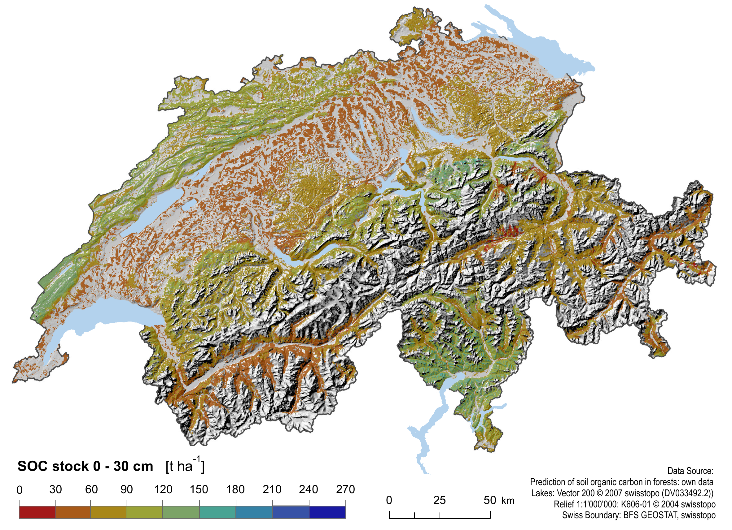
Basis: Punctual kriging and fitted (residual) variogram.
Mean per unit: aproximated by mean of punctual kriging predictions.
Standard errors: “correct” for spatial covariance structure modeled by variogram. I.e. the larger the spatial auto-correlation, the smaller the standard errors for a finite target.
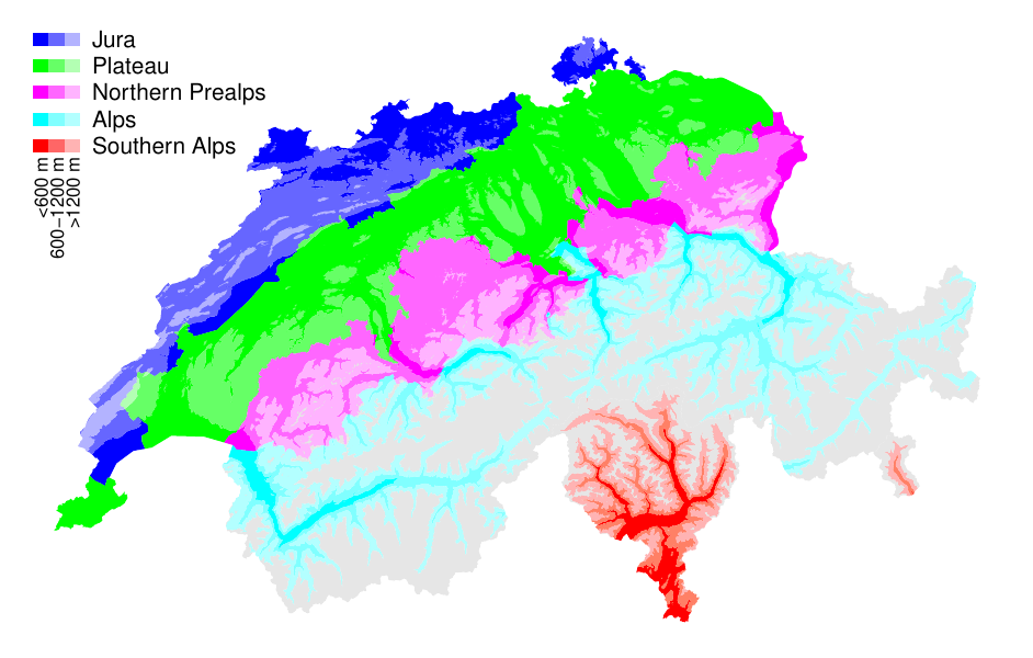
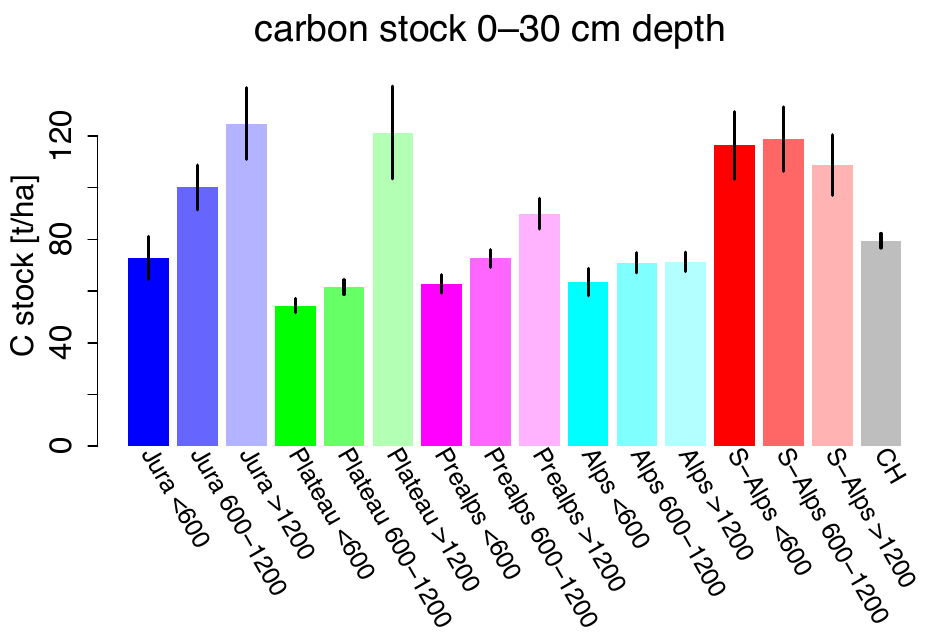
More information in: Oliver + Webster, 2015. / Nussbaum, M., Papritz, A., et al. (2014). Estimating soil organic carbon stocks of Swiss forest soils by robust external-drift kriging. GMD.
Temporal change of soil water storage in a forest. Measurement of soil water storage biweekly during growing season for 2 years (Jost et al., 2005)
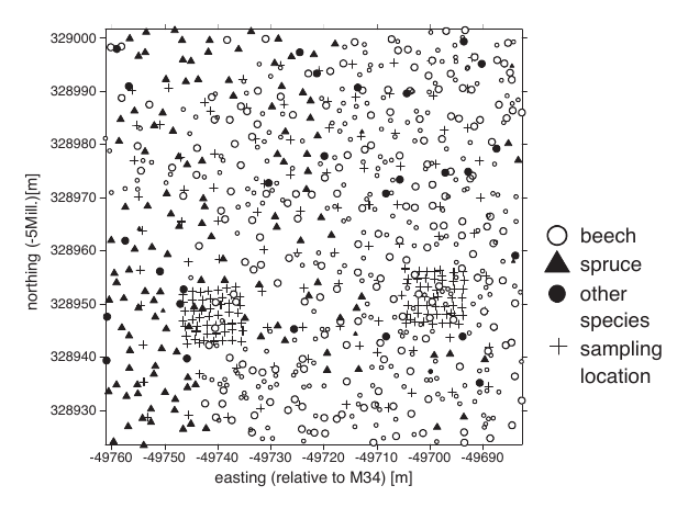
Jost, G., Heuvelink, G. B. M., and Papritz, A. (2005). Analysing thespace-time distribution of soil water storage of a forest ecosystem using spatio-temporal kriging. Geoderma, 128(3–4), 258–273.
Wikle, C. K., Zammit-Mangion, A., and Cressie, N. (2019), Spatio-Temporal Statistics with R, Boca Raton, FL: Chapman & Hall/CRC https://spacetimewithr.org.
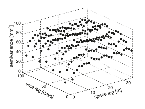
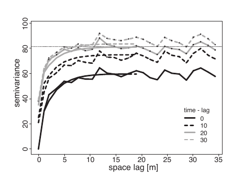
Product-sum covariance model fitted to space-time sample variogram.
Example: Field experiment to compare the yield of 56 varieties of wheat in a randomized block experiment.
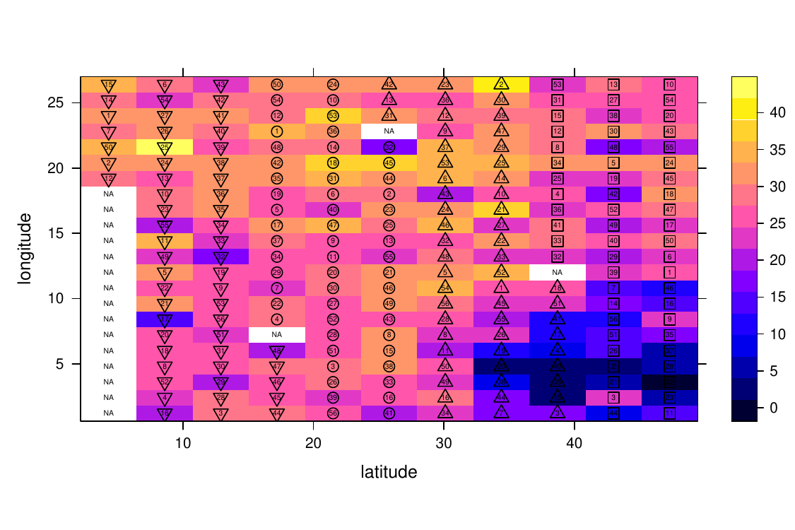
Field experiments in ecology, agriculture, forestry, often give rise to spatial data
Classical analysis of variance of spatial experimental data ignores spatial structure of the data
Blocking and randomisation sometimes not effective to account for natural heterogeneity within experimental site
Residuals often violate independence assumption of classical analysis of variance methods
Explicit consideration of auto-correlation by generalized least squares estimation.
More information on wheat example, p. 260ff in Pinheiro, J. C. and Bates, D. M. (2000). Mixed-Effects Models in S and S-PLUS. Springer.
In areal or lattice data, the domain \(D\) is a fixed countable collection of (regular or irregular) areal units at which variables are observed.
library(sf)
library(mapview)
d <- st_read(system.file("shape/nc.shp", package = "sf"), quiet = TRUE)
mapview(d, zcol = "SID79", map.types = "OpenTopoMap")Number of sudden infant deaths per counties of North Carolina (USA) in 1979.
Cressie N.A.C.: Statistics for Spatial Data. Revised. New York: John Wiley & Sons; 1993.
Certain cells in a section of tissue from a laboratory-induced lymphoma in the kidney of a hamster:
Using this data, we could investigate how different types of cells interact, and what is the relationship between the degree of cell interaction and cancer stage and survival.
library(spatstat)
plot(hamster, main = "Pattern of cells in cancer tissue of a hamster") 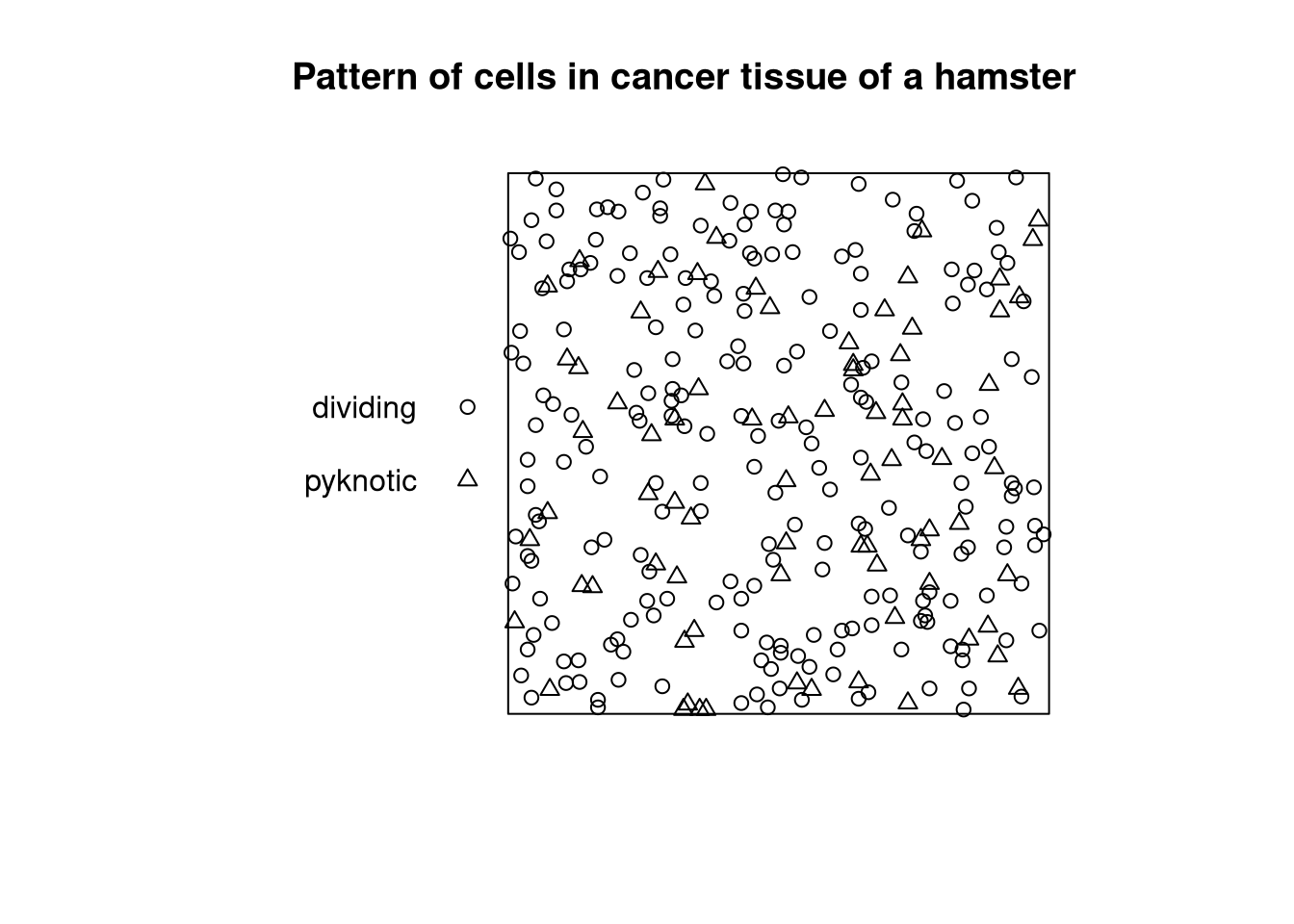
library(spatstat)
plot(lansing, shape="arrows", direction=90, cols=1:6, main = "Locations and botanical classification of trees in Lansing Woods (USA)")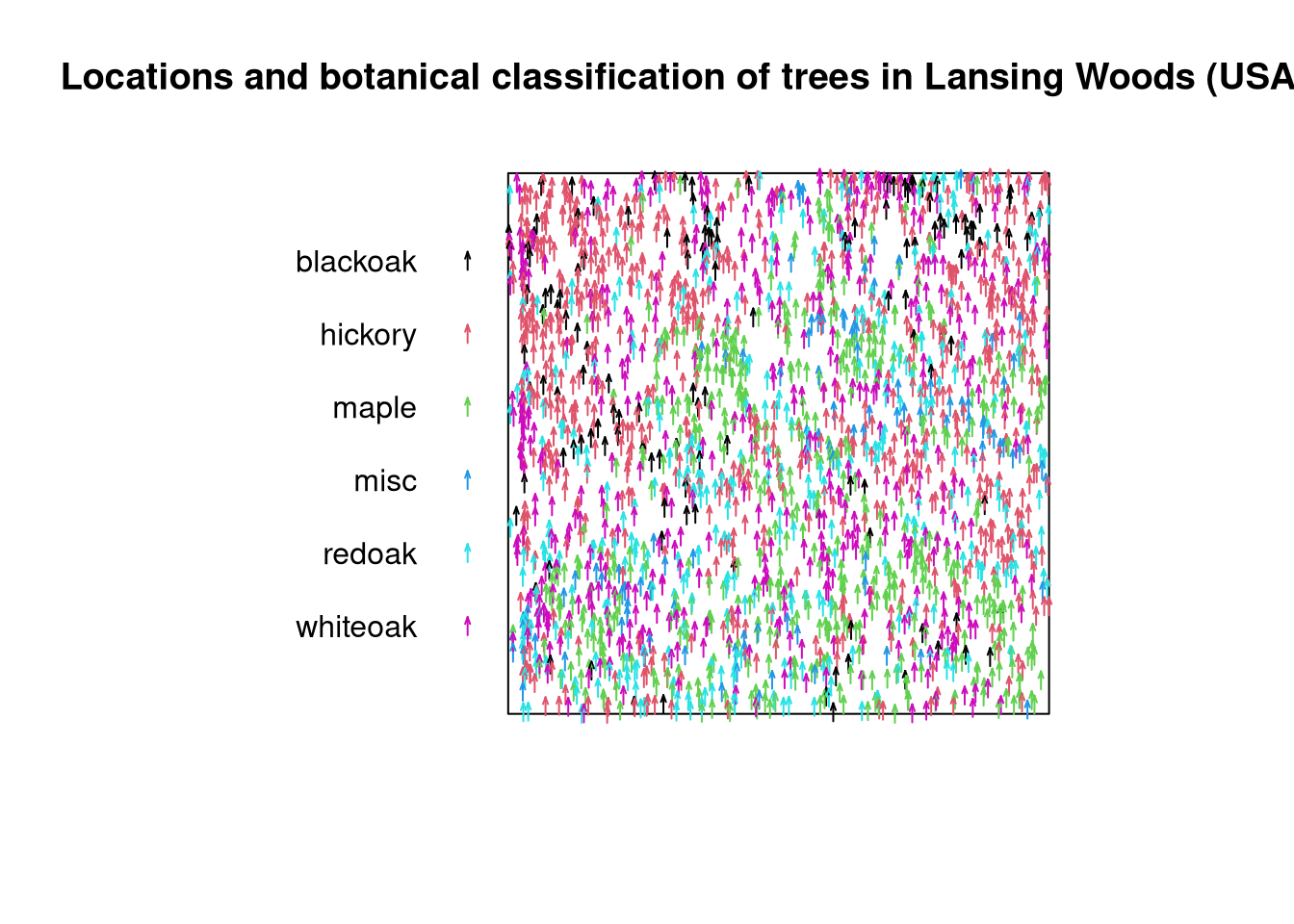
Diggle P.J.: Statistical Analysis of Spatial Point Patterns. 3rd ed. London: Arnold; 2014.