21 Spatial correlation in ML
Download slides PDF
The PDF contains what was shown during the lecture. Some of these websites include additional text in light gray.
21.1 Machine learning for spatial prediction
Advantages
Machine learning (ML) handles today’s requirements for spatial prediction problems well
Large dataset sizes (n observations, n covariates)
Often lowering computational demands
Automatic model selection and building of model structure
Non-linear models, relaxed model assumptions (non-Gaussian error distribution)
Categorical responses (classification)
Uncertainty for point locations
Disadvantages
Spatial auto-correlation is often integrated in ad-hoc manner or not at all
Standard errors for spatial averages only via workaround (e.g. to report quantities per municipality or arable land parcel)
Solved problems within classical geostatistics reoccur for ML
Overview of spatial machine learning
Note: many of the approaches are rather empirically driven “fixes” to include the spatial structure in the data instead of theoretically grounded approaches.
Use spatial information as predictors
Use nearby observations as predictors
Model spatial structure of residuals
Include spatial somehow into algorithm/function
Random forest is widespread for spatial mapping.
Many more or less ad-hoc implementations have been proposed.
→ Subsequent explanations focus on random forest.
21.2 Spatial information as predictors
\(~~Y = f(\mathbf{X}, I) + Z~~\)
where
\(Y\) : observed point data at locations \(i\)
\(f(X)\) : complex function, established by an algorithm using covariates \(\mathbf{X}\)
\(I\) : location \(i\) of the data points
\(Z\) : random error (e.g. measurement error, part we cannot explain with model)
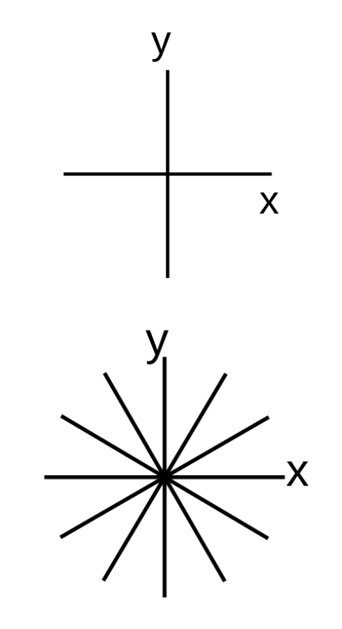
Spatial coordinates axis as covariates
Add x- and y-coordinate axis as additional covariates.
→ Fits (non-linear) spatial trends.
→ Allows random forest to partition study area into smaller sections and fit local models.
Model trend not only North-South and East-West, rotate coordinate axis by \(\alpha\) (in figure: 30° and 60°).
Evaluation
Very simple, works with every ML algorithm
Implicit manner to build local models
for tree based algorithms
- Relates to Universal Kriging
trend model based on coordinates axis
No explicit spatial model nor theoretically grounded.
Can lead to severe artefacts
On predicted maps strange patters can occur such as straight lines or chess board structures.
Relative spatial distances as covariates
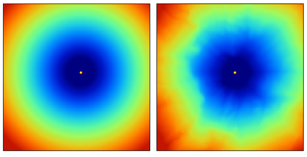
An additional set of covariates is defined based on the relative distance to each observation:
\[ X_G = \{d_{p_1}, d_{p_1}, ..., d_{p_n}\} \]
where \(d_{p_i}\) is the euclidean distance (or any other more complex proximity distance) to the observed location \(p_i\) and \(n\) is the total number of training observations.
→ R packages GSIF, spatialRF.
Example covariate layer for one observation by euclidean distance (left) or travel time distance (right).
Spatial distances as covariates - Evaluation
Evaluation
Works with every ML algorithm.
Relates to kriging as relative distances are included.
Allows for complex anisotropy (directional spatial structure).
No explicit spatial model nor theoretically grounded.
Computational demand for large datasets, study areas: For each \(n\) observations one covariate for the whole study area is generated.
DeepKriging – spatial basis functions + neural network
Use spatial basis functions / spatial representation as part of the neural network (NN).
Embedding layer based on spatial coordinates and multi-resolution radial basis functions added as features.
Basis functions provide spatial patterns at different scales.
NN learns non-linear relations from spatial features to response.
Evaluation
Name somewhat misleading, as it does not explicitly model spatial autocorrelation and produce predictions like kriging
Some statistical motivation, especially for Gaussian case, but no uncertainty estimates
Non-linearity, non-stationarity through interactions
No covariance matrix operations, thus, might be computationally efficient for large datasets
New method, its usefulness still needs to be proven, no mature software yet
21.3 Nearby observations as predictors
\(~~Y(i_0) = f(~\mathbf{X}(i_0), g(Y(i_{1..m})~) + Z\)
where
\(Y(i_0)\) : response observation \(Y\) at location \(i_0\)
\(\mathbf{X}(i_0)\) : predictors at location \(i_0\)
\(Y(i_{1..m})\) : response values \(Y\) of neighboring observations at locations \(i_1\) up to the defined neighborhood \(m\)
\(g()\) : optional function that is applied to neighboring observations \(Y_{i}\)
Spatial neighbor values and distances as covariates
Include observed values from \(n\) nearest locations and distances to these locations.
For each \(n\) nearest neighbor 2 colums are added as covariates:
- value at \(n\)th nearest observation
- distance corresponding to the location contributing the observed value
\(n\) is a tuning parameter.
→ R package RFSI
Evaluation
Works with every ML algorithm.
Recycles the idea of computing weighted means of the neighbouring observations.
Relates to lagged response values in time series analysis.
No explicit spatial model nor theoretically grounded.
Predictive performance benefit unclear.
On the 2nd item: Measurements of previous time steps are included to predict the current time step.
Spatial predictors constructed from neighbouring observations
Create predictors by using response values \(Y\) to create continuous surfaces.
Options:
- Local averages
- Distance-weighted observations, e.g. Inverse Distance Weighting
- Ordinary kriging from observations, e.g. leave-one-out ordinary kriging (LOO-OK)
Evaluation
Works with every ML algorithm.
Possibly computationally inefficient (LOO-OK).
Danger of data leakage in validation (e.g. cross-validation)
No explicit spatial model nor theoretically grounded.
21.4 Model spatial structure of residuals
\(Y = f(\mathbf{X}) + E + Z\)
where
\(f(\mathbf{X})\) : general trend function modeled with covariates \(\mathbf{X}\) (raster data) where \(f()\) can be any kind of function e.g. built by a machine learning algorithm
\(E\) : small scale fluctuations, spatial autocorrelation modeled by ordinary kriging
ML models what covariates explain; geostatistics handles the spatially correlated remainder. Often termed regression kriging or residual kriging.
Two step approach:
Fit non-spatial model, compute its residuals.
Fit ordinary kriging to residuals.
Predictions are a sum of model outputs from (1) and (2).
Trend function could also be a linear model (see e.g. analysis of Wolfcamp data in Geostatistics section).
Regression kriging - Evaluation
Evaluation
Works with every ML algorithm
Separates the prediction into an explainable component and a spatially correlated residual.
Non-spatial method often ignores spatial correlation in model fit.
Quantification of prediction uncertainty remains difficult.
Some challenges with kriging are re-introduced (stationarity, Gaussian assumptions).
21.5 Make prediction function spatial
\(~~Y = f_i(\mathbf{X}) + Z\)
where
\(f_i()\) : complex function where locations \(i\) of observations are used to establish the function
Several directions:
- Geographically varying models
- geographically weighted models
- smooth spatial surfaces
- Spatial covariance enters model fitting
Geographically weighted models
Geographically weighted regression (GWR)
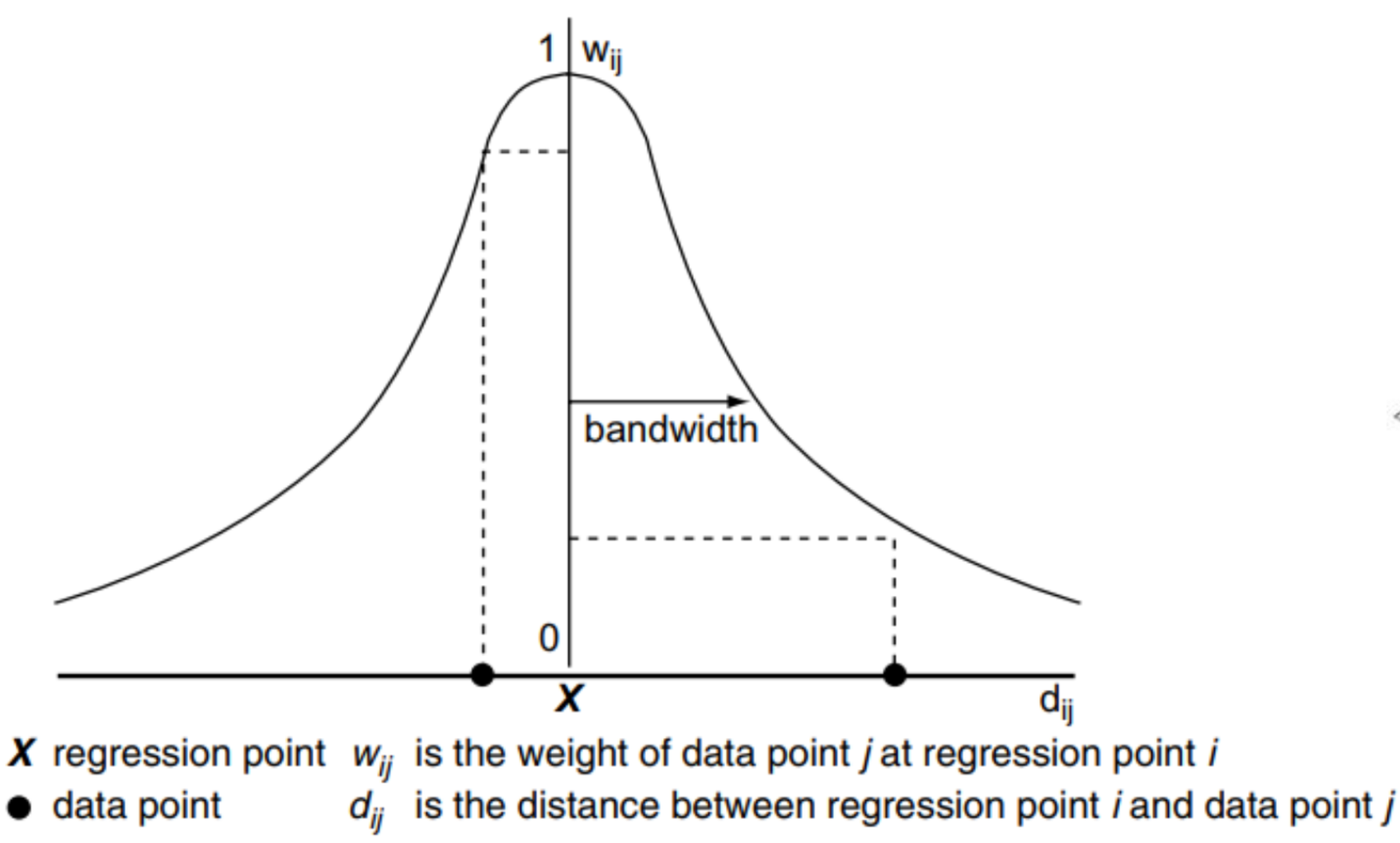
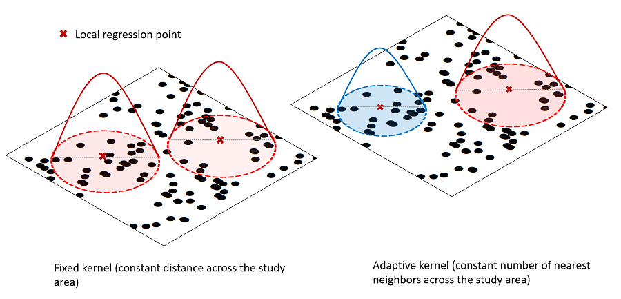
Local linear models built on moving window across study area.
Kernel to fit local models: fixed distance or fixed number of observations.
Model choices: Shape of weighting scheme and kernel bandwidth (tuning parameter)
Was expanded to fit local random forest
Geographically weighted models - Evaluation
Evaluation
Contrasting idea to kriging: Does not model spatial autocorreleation, but local relationships with predictors → spatially varying coefficients/models.
Quite widespread method in some fields (human geography, biodiversity studies)
Residual spatial autocorrelation is not not modeled, i.e. assumed to be captured by local models.
Likely sensitive to outliers, stability of local models?
If used with linear models: huge number of linear models with non-verified assumptions (residual diagnostics) and possible multi-collinearity problems.
Mapping of local relationships significance, however, prone to over-interpretation and multiple testing problem
Huge number of models, quickly computationally non-feasible
Predictions are created from a local model that is fitted at every pixel. For each pixel, the neighbourhood is determined, a local model is established and the prediction computed.
Smooth surface of coordinates
Works for Generalized Additive Models (GAM), i.e. fitted by boosting algorithm
Spatial auto-correlation can be modeled by including a “smooth spatial surface”
Non-stationary covariate effects by interactions with surface (tensor splines)
→ R packages mgcv, mboost, geoGAM
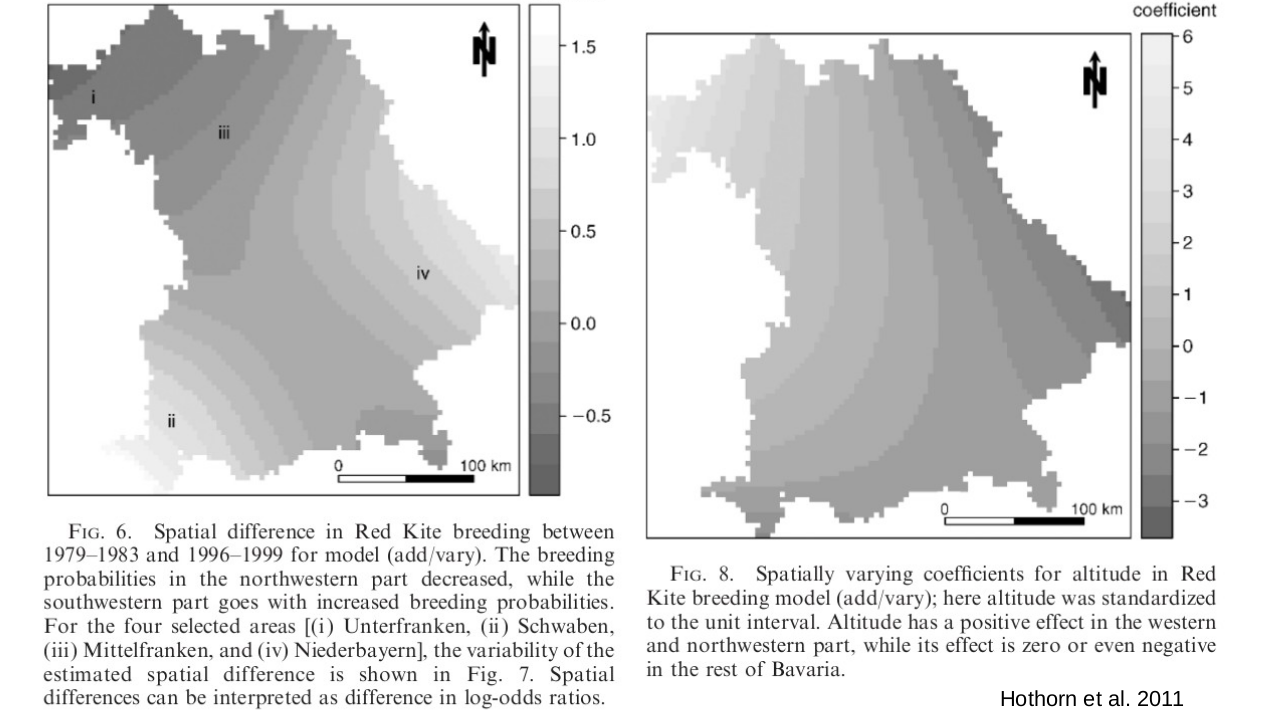
Evaluation
Smooth local surfaces defined globally, thus better model interpretation (vs. GWR).
Smooth surfaces are estimated during model fitting (opposed to observation derived predictors).
Choice of degrees of freedom for splines surfaces unclear → overfitting or underfitting.
Granularity of smooth spatial surface defines model for spatial autocorrelation.
Might overfit or if constrained not catch the spatial structure in the data.
RF-GLS: Generalized least squares random forest
Use spatial covariance to fit random forest (RF) using Generalized Least Squares (GLS).
Idea:
Fit an ordinary RF initially.
Estimate spatial covariance parameters (variogram) from RF residuals.
Use estimated covariance matrix in the RF-GLS fitting:
- resampling corrected by covariance structure
- spatially adjusted split criterion (GLS fit)
- spatially adjusted node estimates / predictions (GLS model estimates)
For prediction at new locations, RF-GLS can combine mean predictions (GLS predictions, not mean of nodes) with kriging predictions based on the estimated variogram.
→ R package RandomForestsGLS
RF-GLS builds in established concepts into the RF algorithm, such as the generalized least squares fitting.
The resampling procedure (bootstrap) used in normal RF is based on the assumption of independent observations. In RF-GLS decorrelated contrasts are used. A contrast is essentially a linear combination of observations. The covariance-based transformation leads to an approximately uncorrelated outcome.
Similar to REML fitting geostatistical model with external drift. But, no iterative fitting. Variogram parameters are estimated once from residuals of an initial RF and then treated as fixed when fitting the RF-GLS.
RF-GLS – Evaluation
Evaluation
Introduces geostatistical model into the linear fitting part of random forest.
So far most statistically principled spatial adaptation of ML.
Needs specification of e.g. variogram function → possibly difficult for pure ML users
Computationally very heavy, variogram needs to be fitted at every tree split.
Evidence that model performance is better than conventional RF, but still matter of ongoing research.
The covariance matrix for the GLS fitting and prediction is done only once for the whole forest. However, RF-GLS is computationally heavy, because a large number of candidate splits have to be evaluated at each tree node. The contributing observations change for each split, which does not allow for easy updating of the means/sums accross nodes and thus it cannot be profited from the fast random forest implementations. RF-GLS uses a sparse matrix approximation (NNGP approximation) to alleviate this, but even with this it remains significantly slower compared to other spatial RF adaptations (10.1016/j.envsoft.2025.106626).
Spatial Neuronal Networks (NN) – 1
NN-GLS – neural network + geostatistical model
Replace the linear mean \(X\beta\) in geostatistical model by a neural network \(f_\theta(X)\)
NN with covariance matrix in loss function (GLS)
Spatial covariance explicitly affects estimation, related to RF-GLS.
Covariance is part of model rather than being represented by spatial predictors. Unlike RF-GLS, covariance parameters are updated during NN training.
Retains geostatistical prediction: predictions at new locations can be obtained by kriging, including the spatial residual component.
Statistically principled, scaleable implementation → Promising approach, however, not yet mature.
→ Python implementation geospaNN
Spatial Neuronal Networks (NN) – 2
Convolutional Neural Networks (CNN) — spatial structure through the architecture
Convolutional layers exploit local neighbourhoods: predictions depend on patterns in nearby pixels.
Spatial dependence encoded by network architecture and convolution kernels, rather than by an explicit covariance function.
Established for raster/grid data (images), some applications for irregular point observations with neighbourhood tiles as model inputs
Network learns spatial filters from data, rather than specifying a covariance model.
21.6 Spatial machine learning – summary
No method stands out, currently no fully satisfactory solution.
Many proposed methods are merely ad-hoc.
RandomForestGLS as promising solution, but computationally heavy.
Neuronal network approaches under development.
You could also just keep it simple: Use rotated coordinate axis, but carefully evaluate your result.