28 Lab: Spatial sampling

Download R Code

28.1 Create sampling design for training

In this section we will create a Feature Coverage Sampling Design for the La Réunion dataset.

Installation and data download

Install required R packages

l.p <- c("terra", "sf", "fields", "ranger", "ggplot2") # optional: "mapview"
install.packages(l.p)

Download dataset

Download link

This zip contains a folder terrain with derivatives from the elevation model and folder soil with a map of soil organic carbon stocks extracted from the global overview soil map SoilGrids.

Unpack the folder into a folder called datasets.

Prepare data

Read in data and check content

library(terra)
library(sf)
library(fields)

# set working directory to folder above "data"
r.dem <- rast("datasets/lareunion/data/terrain/reunion_30m.tif")
r.dem

class       : SpatRaster 
size        : 769, 667, 1  (nrow, ncol, nlyr)
resolution  : 30, 30  (x, y)
extent      : 330000, 350010, 7669992, 7693062  (xmin, xmax, ymin, ymax)
coord. ref. : WGS 84 / UTM zone 40S (EPSG:32740) 
source      : reunion_30m.tif 
name        : reunion_30m 
min value   :   -3.551687 
max value   : 2274.301270

Create first display

plot(r.dem)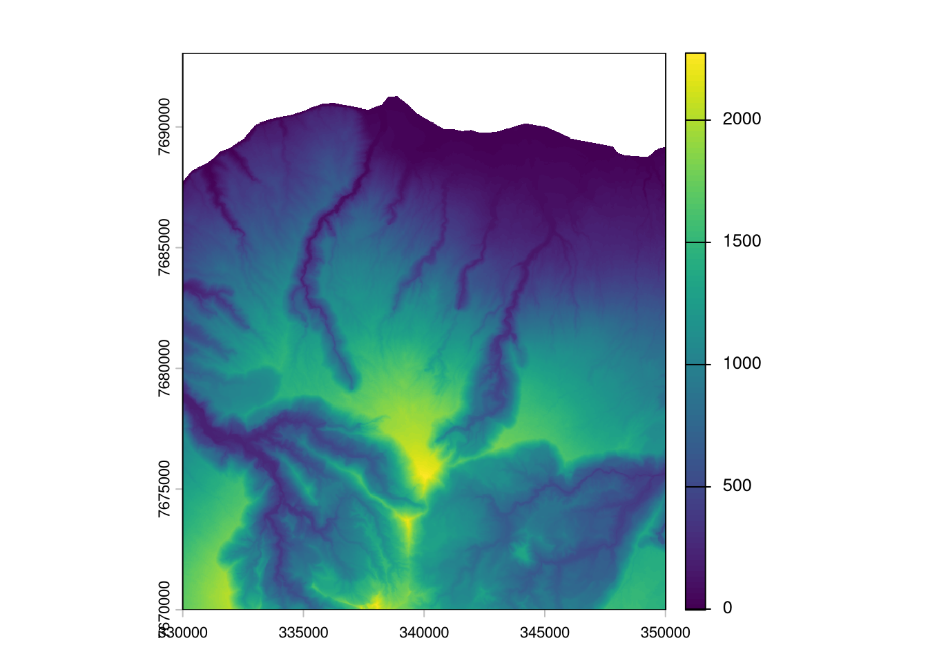

Select variables for sampling design and transform into data.frame

For now we decided to use elevation (reunion_30m.tif), slope computed on 100 by 100 m pixels (slope100m-perc.tif) and a topographic position index calculated at 900 m diameter (tpi_900m.tif).

# create a list of file names
l.rast <- paste0("datasets/lareunion/data/terrain/", c("reunion_30m.tif", "slope100m-perc.tif", "tpi_900m.tif"))

# create a raster stack
r.stack <- rast(l.rast)

# create a data frame, each row corresponds to a pixel
d.pixels <- as.data.frame(r.stack, xy = T, na.rm = F)
str(d.pixels)

'data.frame':   512923 obs. of  5 variables:
 $ x             : num  330015 330045 330075 330105 330135 ...
 $ y             : num  7693047 7693047 7693047 7693047 7693047 ...
 $ reunion_30m   : num  NA NA NA NA NA NA NA NA NA NA ...
 $ slope100m-perc: num  NA NA NA NA NA NA NA NA NA NA ...
 $ tpi_900m      : num  NA NA NA NA NA NA NA NA NA NA ...

Select relevant pixels

To reduce computational load and ensure a minimal distance between sampling points we use every second pixel (60 m distance).

# only use every second pixel, ensures 60 m distance between sampling points
t.sel.x <- d.pixels$x %in% seq(min(d.pixels$x), max(d.pixels$x), by = res(r.stack)[1]*2)
t.sel.y <- d.pixels$y %in% seq(min(d.pixels$y), max(d.pixels$y), by = res(r.stack)[1]*2)

# remove NA, and remove every second pixel
d.pixels <- d.pixels[ complete.cases(d.pixels) & t.sel.x & t.sel.y, ]

str(d.pixels)

'data.frame':   102777 obs. of  5 variables:
 $ x             : num  338655 338715 338775 338835 338655 ...
 $ y             : num  7690707 7690707 7690707 7690707 7690647 ...
 $ reunion_30m   : num  19.7 18.8 18.3 17.4 21.9 ...
 $ slope100m-perc: num  0.0443 0.0448 0.0439 0.041 0.0477 ...
 $ tpi_900m      : num  2.81 2.02 1.76 2.21 2.9 ...

k-means clustering

Form as many clusters as we like to have samples. For the clusering we use the 3 variables defined above, but also the spatial coordinates to ensure equal spatial coverage.

# scale variables and round to 5 digits to make clustering more stable
d.pixels.sc <- round(scale(d.pixels), 5)

# set seed for reproducibility 
set.seed(11)
# k-means clustering, with centers = numbers of samples to plan
m.kmeans <- kmeans(d.pixels.sc, centers = 150, iter.max = 50)

# number of pixels per cluster
m.kmeans$size

  [1]  334  634  385  971  406  249  444  483  479  601  451 1090  893  578  952
 [16]  517  769  197  624  704 1001  590  510  682  673  949  652  933  308  668
 [31]  461  796  431  742  849  809  509  473  678 1172  506 1132 1032 1409  739
 [46]  439  652  467  831  534  545  415  808  276  420  882  191  851  778 1579
 [61]  709  634  717  931 1625  333  411  815  436  579  622  821 1033  399  973
 [76]  788  511  445  358  661  521 1150  467  513 1142  620  900  397  770  706
 [91]  629  408  694  296  499  737 1006  904  427  603  573 1284  702  544 1179
[106]  913  437 1015  764  835  532  658  826  620 1409 1036  883  797  314  512
[121]  520  799  363 1001  694 1222  605  471  605  825 1026  202  362  567  463
[136]  898  447  955  435 1195  719  367  705  593  991  892  293  875  385  146

Select sampling point

Select pixel that is closest to cluster center (cluster center is a calculated mean).

# extract real points closest to cluster center
m.dist <- rdist(d.pixels.sc, m.kmeans$centers)
# select row indices 
idx <- apply(m.dist, 2, which.min)

d.sample <- d.pixels[idx, 1:2]

# create sample IDs
d.sample$id <- paste0("train_", 1:nrow(d.sample))

# create a spatial points object and save to Geopackage
v.sample <- st_as_sf(d.sample, coords = c("x", "y"), crs = 32740)
write_sf(v.sample, "datasets/lareunion/results/fsc_design_150.gpkg")

v.sample

Simple feature collection with 150 features and 1 field
Geometry type: POINT
Dimension:     XY
Bounding box:  xmin: 330675 ymin: 7671147 xmax: 349335 ymax: 7689387
Projected CRS: WGS 84 / UTM zone 40S
First 10 features:
             id               geometry
357815  train_1 POINT (339075 7676967)
273509  train_2 POINT (331155 7680747)
177921  train_3 POINT (344955 7685067)
404519  train_4 POINT (339495 7674867)
261875  train_5 POINT (342315 7681287)
343079  train_6 POINT (337215 7677627)
188259  train_7 POINT (334935 7684587)
251163  train_8 POINT (341115 7681767)
360439  train_9 POINT (337755 7676847)
452723 train_10 POINT (344895 7672707)

Display created sampling points

library(mapview)
mapviewOptions(basemaps = c("OpenStreetMap", "OpenTopoMap", "Esri.WorldImagery")) # default map requires an API key
mapview(v.sample)

Create a map of cluster zones

Create predictions of clustered areas.

# extract cluster for each pixel
d.pixels$clusters <- fitted(m.kmeans, "classes")
# create a raster object 
r.clusters <- rast(d.pixels[, c("x", "y", "clusters")], type="xyz", crs= "epsg:32740")
writeRaster(r.clusters, filename = "datasets/lareunion/results/fsc_design_150_clusters.tif", overwrite = T)
plot(r.clusters)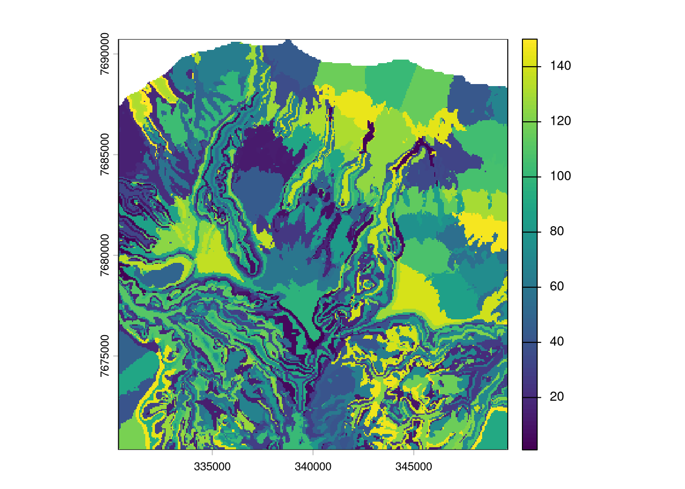

Tasks

Task 1

Display the created sampling points and cluster zones in QGis. Also add background map. Verify your result. Would you pass it to the surveyors? Or what would you improve?

Task 2

Remove the spatial coordinates from the clustering. Do you see a difference and why?

Task 3

Change other criteria such as the number of sampling points or chose other variables for the clustering. Observe the changes and compare with how you would manually place sampling points on a map.

28.2 Create sampling for map validation

Now we create a stratified random sample to estimate the map error.

Form strata

As we have no further information on the distribution of the map errors we assume elevation is a relevant factor. We plan 30 sampling points and from 3 strata, thus 10 random points per stratum.

# use elevation as strata, from 3 strata
t.breaks <- quantile(d.pixels$reunion_30m, probs = seq(0,1,1/3))
d.pixels$strata <- cut(d.pixels$reunion_30m, breaks = t.breaks, labels = 1:3)

# check if it worked
table(d.pixels$strata)


    1     2     3 
34258 34259 34259

Plot maps of strata

# save strata map
r.strata <- classify(r.stack[[1]], rcl = t.breaks)
writeRaster(r.strata, filename = "datasets/lareunion/results/strs_design_3_strata.tif", overwrite = T)

plot(r.strata)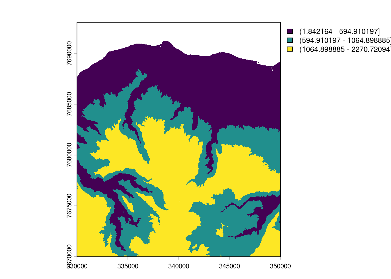

Select random samples per stratum

set.seed(1)

# apply random selection of 10 points for each strata
l.sample.rows <- lapply(c("1", "2", "3"), function(stratum){
  # select relevant row names 
  l.row <- rownames(d.pixels[ d.pixels$strata == stratum, ])
  # randomly select 10 of the row names
  l.rs <- sample(l.row, 10)
  return(l.rs)
})

# select corresponding pixel 
d.sample <- d.pixels[ unlist(l.sample.rows), ]

# check if number per strata are ok
table(d.sample$strata)


 1  2  3 
10 10 10

# create sample IDs
d.sample$id <- paste0("val_", 1:nrow(d.sample))

v.validation <- st_as_sf(d.sample[, c(1:2,5)], coords = c("x", "y"), crs = 32740)
write_sf(v.validation, "datasets/lareunion/results/strs_design_30.gpkg")

Display results

mapview(v.validation)

Tasks

Task 1

Is the distribution of point locations as you would expect it? Change the seed. What happens?

Task 2

The Horvitz-Thompson estimator has not been used in this section. Does it apply to this case? Where does it need to be applied?

Task 3

Create strata that have equal area coverage. For this create a k-means clustering (with e.g. k = 3) just using the coordinates. For each clustered zone again take a random sample.

28.3 Use sampling designs for mapping

Soil map (instead of real sampling)

In this section we use the created sampling desings to create a map of soil organic stocks and to validate map accuracy. We imitate real sampling by reading out values from the global overview soil map SoilGrids.

r.soc <- rast("datasets/lareunion/data/soil/soilgrids_SOCstock_0-30_mean30mSmooth.tif")
plot(r.soc)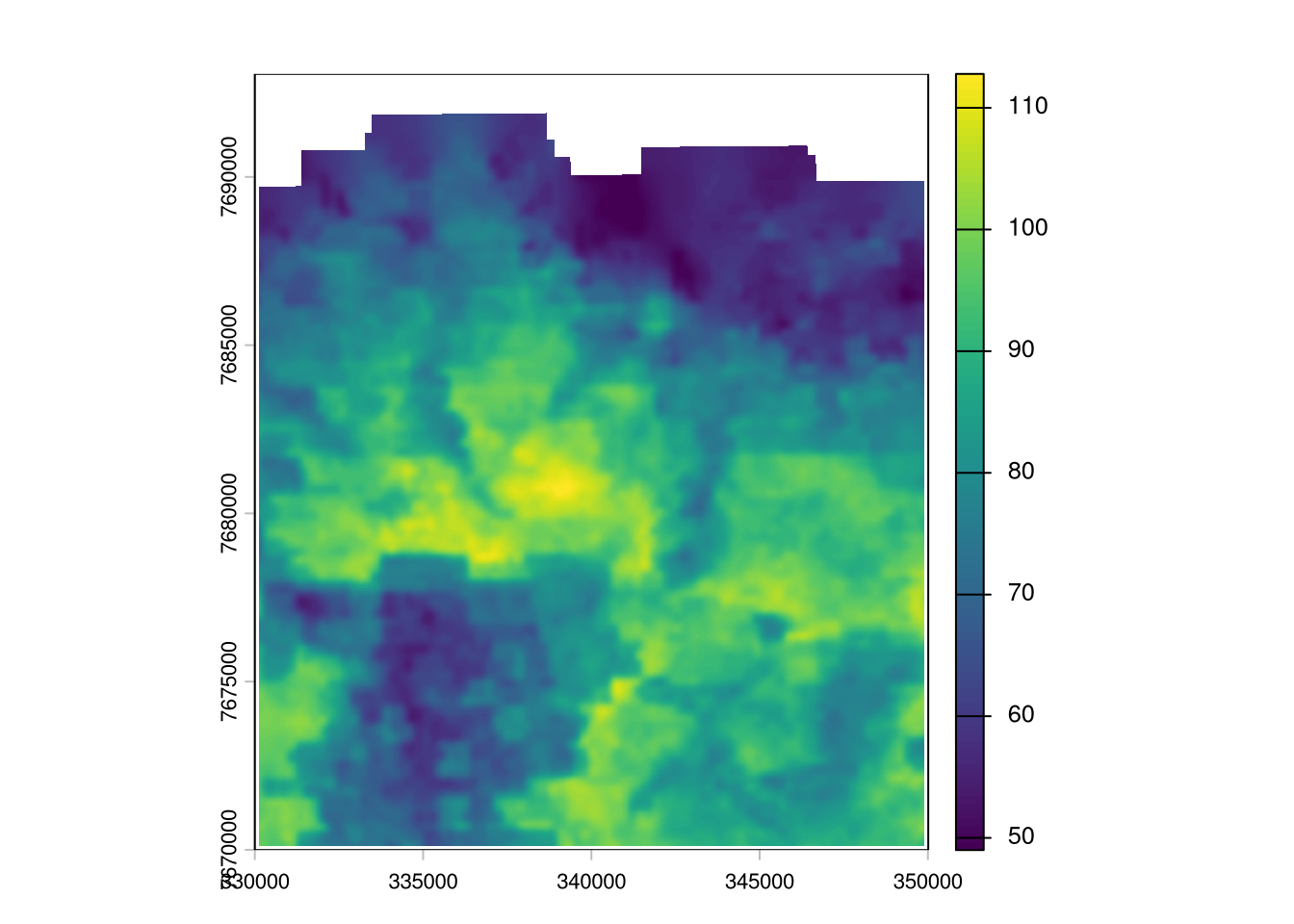

Prepare response data

library(ranger)
library(ggplot2)

l.rast <- list.files("datasets/lareunion/data/terrain/", pattern = ".tif$", full.names = T)
r.stack <- rast(l.rast)

v.samples <- st_read("datasets/lareunion/results/fsc_design_150.gpkg")

Reading layer `fsc_design_150' from data source 
  `/home/nussbaum/repos-uu/spatialstats-web/course-website/datasets/lareunion/results/fsc_design_150.gpkg' 
  using driver `GPKG'
Simple feature collection with 150 features and 1 field
Geometry type: POINT
Dimension:     XY
Bounding box:  xmin: 330675 ymin: 7671147 xmax: 349335 ymax: 7689387
Projected CRS: WGS 84 / UTM zone 40S

# read response value 
# (in a real project, we would read the values from the lab measured on soil samples)
d.SOCstock <- extract(r.soc, v.samples)

str(d.SOCstock)

'data.frame':   150 obs. of  2 variables:
 $ ID                                   : num  1 2 3 4 5 6 7 8 9 10 ...
 $ soilgrids_SOCstock_0-30_mean30mSmooth: num  76.2 79.4 68.7 80.6 88.2 ...

Prepare predictor data

# read predictor values at sampling locations 
d.predictors <- extract(r.stack, v.samples)

str(d.predictors)

'data.frame':   150 obs. of  35 variables:
 $ ID              : num  1 2 3 4 5 6 7 8 9 10 ...
 $ asp_eness30m    : num  -0.948 0.167 -0.273 -0.988 0.372 ...
 $ asp_nness30m    : num  -0.2546 0.982 0.953 0.0444 0.9281 ...
 $ curv100m        : num  0.00702 0.00803 -0.00431 -0.00452 0.00263 ...
 $ curv30m         : num  0.009431 0.019959 -0.022337 -0.029317 0.000387 ...
 $ curvplan100m    : num  0.000514 0.003546 -0.026976 -0.001553 0.005157 ...
 $ curvplan30m     : num  -0.01869 0.02169 0.008 -0.00652 -0.00581 ...
 $ curvprof100m    : num  0.002752 0.000615 -0.000834 -0.000241 -0.000348 ...
 $ curvprof30m     : num  0.007082 -0.001764 -0.011551 -0.000702 0.001665 ...
 $ heignor100m     : num  0.939 0.695 0.112 0.407 0.918 ...
 $ heignor30m      : num  0.9834 0.8409 0.0765 0.2528 0.8918 ...
 $ heigslope100m   : num  724.8 161.9 26.6 267.7 403.3 ...
 $ heigslope30m    : num  812.9 174.1 13.6 139.7 346.3 ...
 $ heigstand100m   : num  1887.2 612.9 15.2 625.9 987.7 ...
 $ heigstand30m    : num  1991.43 744.34 6.94 378.71 960.64 ...
 $ heigval100m     : num  46.1 69.4 212.7 389.6 35 ...
 $ heigval30m      : num  13.7 32.9 164 412.8 42 ...
 $ mpi100m_150     : num  0.0669 0.1218 0.1837 0.3102 0.0799 ...
 $ mpi30m_150      : num  0.0173 0.144 0.2481 0.528 0.1072 ...
 $ mrrtf100m       : num  8.22e-02 3.26e-10 2.58e-07 4.70e-14 4.74e-06 ...
 $ mrrtf30m        : num  1.92e-03 2.46e-10 6.74e-09 2.22e-16 6.11e-05 ...
 $ mrvbf100m       : num  3.01e-04 1.14e-11 4.12e-03 1.12e-12 5.24e-08 ...
 $ mrvbf30m        : num  3.09e-05 2.17e-11 1.62e-06 2.91e-14 6.56e-05 ...
 $ reunion_30m     : num  2025 886 134 1508 1078 ...
 $ slope100m-perc  : num  0.403 0.64 0.265 0.8 0.356 ...
 $ slope30m-perc   : num  0.137 0.531 0.373 1.001 0.282 ...
 $ tpi_270m        : num  28.45 27.66 -23.75 -33.43 7.11 ...
 $ tpi_900m        : num  96.1 68.9 -50.4 -36.4 83.4 ...
 $ tri100m         : num  182 141 69 251 147 ...
 $ tri30m          : num  52.4 65.4 39.3 83.2 30.6 ...
 $ TWIsaga100m_s100: num  6.94 6.11 9.45 6.86 6.22 ...
 $ TWIsaga100m     : num  6.74 5.61 10.01 7.16 6.24 ...
 $ TWIsaga30m      : num  6.44 4.63 10.88 7.45 6.79 ...
 $ vrm100m         : num  0.0868 0.116 0.0424 0.087 0.1374 ...
 $ vrm30m          : num  0.0868 0.0627 0.1038 0.0644 0.0365 ...

Fit random forest

Quick and dirty random forest model fit.

## fit RF model
m.rf <- ranger(y = d.SOCstock$`soilgrids_SOCstock_0-30_mean30mSmooth`,
               x = d.predictors[,-c(1)], # do not use ID
               importance ="permutation")
m.rf

Ranger result

Call:
 ranger(y = d.SOCstock$`soilgrids_SOCstock_0-30_mean30mSmooth`,      x = d.predictors[, -c(1)], importance = "permutation") 

Type:                             Regression 
Number of trees:                  500 
Sample size:                      150 
Number of independent variables:  34 
Mtry:                             5 
Target node size:                 5 
Variable importance mode:         permutation 
Splitrule:                        variance 
OOB prediction error (MSE):       77.93772 
R squared (OOB):                  0.5437146

Predictor importance

t.importance <- importance(m.rf)

par(oma = c(2,10,2,2))
barplot(t.importance[order(t.importance)], horiz= T, las = 1, cex.names = 0.6)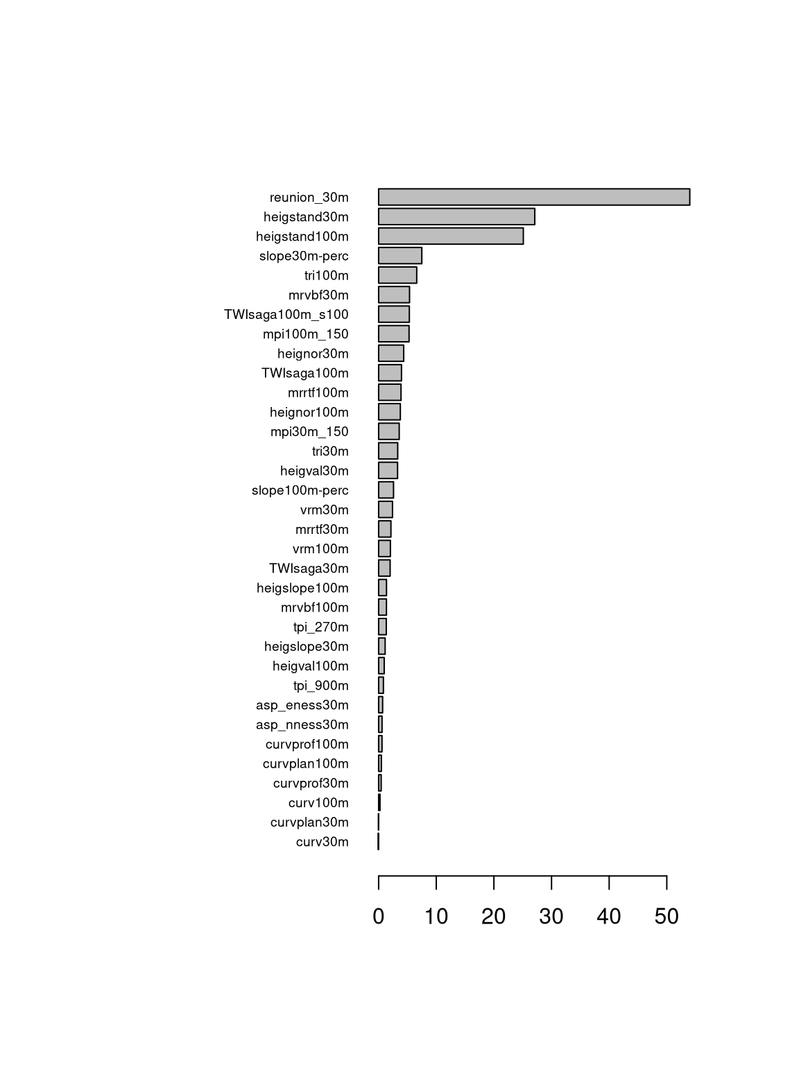

Evaluate map accuracy

Predict on validation sample

## Compute validation stats 
v.validation <- st_read("datasets/lareunion/results/strs_design_30.gpkg")

Reading layer `strs_design_30' from data source 
  `/home/nussbaum/repos-uu/spatialstats-web/course-website/datasets/lareunion/results/strs_design_30.gpkg' 
  using driver `GPKG'
Simple feature collection with 30 features and 1 field
Geometry type: POINT
Dimension:     XY
Bounding box:  xmin: 330375 ymin: 7670487 xmax: 349095 ymax: 7688847
Projected CRS: WGS 84 / UTM zone 40S

d.predictors.val <- extract(r.stack, v.validation)
d.SOCstock.val <- extract(r.soc, v.validation)

d.SOCstock.val$predictions <- predict(m.rf, d.predictors.val)$prediction
summary(d.SOCstock.val$predictions)

   Min. 1st Qu.  Median    Mean 3rd Qu.    Max. 
  55.82   74.61   80.41   80.40   88.60   91.93

Validation statistics

# compute marginal bias (positive values: overestimation, negative values: underestimation)
error <- d.SOCstock.val$`soilgrids_SOCstock_0-30_mean30mSmooth` - d.SOCstock.val$predictions
mean(-error)

[1] -1.942238

# RMSE
sqrt(mean(error^2))

[1] 6.949492

# R2, computed as skill score / model efficiency coefficient 
obs <- d.SOCstock.val$`soilgrids_SOCstock_0-30_mean30mSmooth`
1 - ( sum( error^2 ) / sum( (obs - mean(obs))^2 ) )

[1] 0.711062

Validation scatterplot

library(ggplot2)
ggplot(d.SOCstock.val, aes(predictions, `soilgrids_SOCstock_0-30_mean30mSmooth`)) +
  geom_point(size = 2) + ylim(52,108) + xlim(52,108) +
  xlab(expression("predicted SOC stocks [t" ~ha^-1~"]")) +
  ylab(expression("observed SOC stocks [t" ~ha^-1~"]")) +
  stat_smooth(se = FALSE, span = 1.5) + 
  geom_abline (slope=1, linetype = "dashed", color="black") +
  theme_minimal()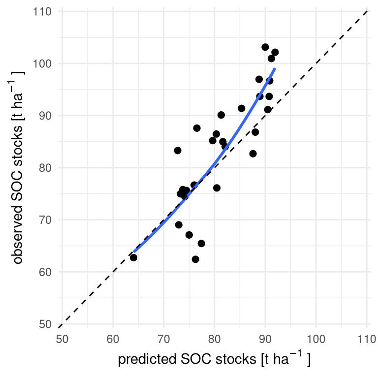

Create spatial predictions

# create a data frame, each row corresponds to a pixel
d.pixels <- as.data.frame(r.stack, xy = T, na.rm = F)

# remove NA
d.pixels <- d.pixels[ complete.cases(d.pixels), ]

# check if we have all predictors, list missing columns 
names(importance(m.rf))[ !names(importance(m.rf)) %in% names(d.pixels) ]

character(0)

# predict using ranger object 
d.pixels$SOCstock_predictions <- predict(m.rf, d.pixels)$predictions

# create a raster object and save 
r.pred <- rast(d.pixels[, c("x", "y", "SOCstock_predictions")], type="xyz", crs= "epsg:32740")
writeRaster(r.pred, filename = "datasets/lareunion/results/predicted_SOC_stocks.tif", overwrite = T)

Display results

plot(r.pred)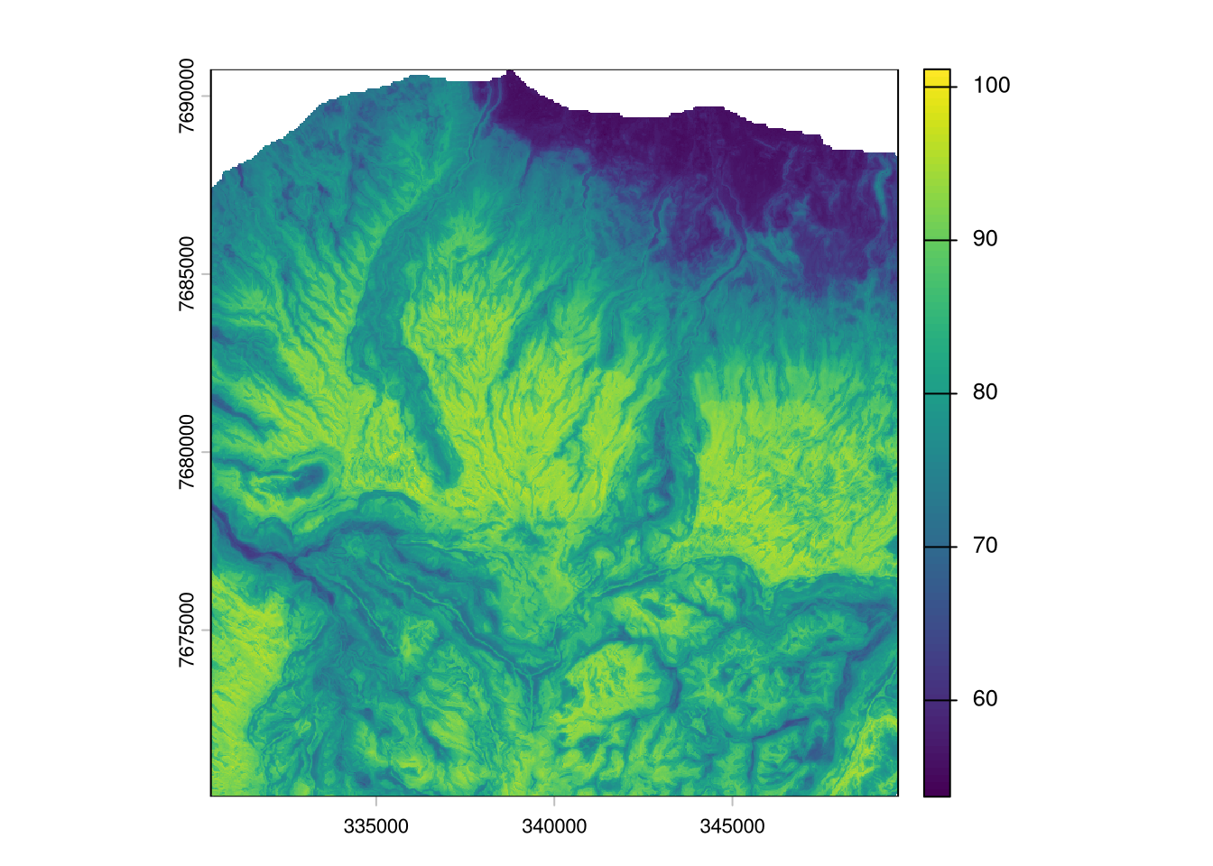

Tasks

Task 1

Compare the created map to the soil organic carbon stock map from SoilGrids. How well do they align? Where are major differences? And which map would you trust more as an end-user?