17 Introduction to Machine Learning

Download slides PDF

The PDF contains what was shown during the lecture. Some of these websites include additional text in light gray.

e-Lecture video

This lecture is available as recording.

17.1 What is Machine Learning (ML)?

Machine learning (ML): algorithms that learn patterns from data to make predictions or decisions.
Core idea: use data to approximate a function (f: X Y) instead of hand-crafting rules.
Typical tasks: regression (continuous outcome Y), classification (categorical outcome Y), clustering (no outcome).

ML Paradigms

Supervised learning: data with target variable (X, Y) → learn to predict Y from X.
Unsupervised learning: only X → discover structure (clusters, embeddings).
Reinforcement learning: agents learn by interacting with an environment and receiving rewards.

17.2 How to balance model complexity?

Illustration of Bias-Variance trade-off

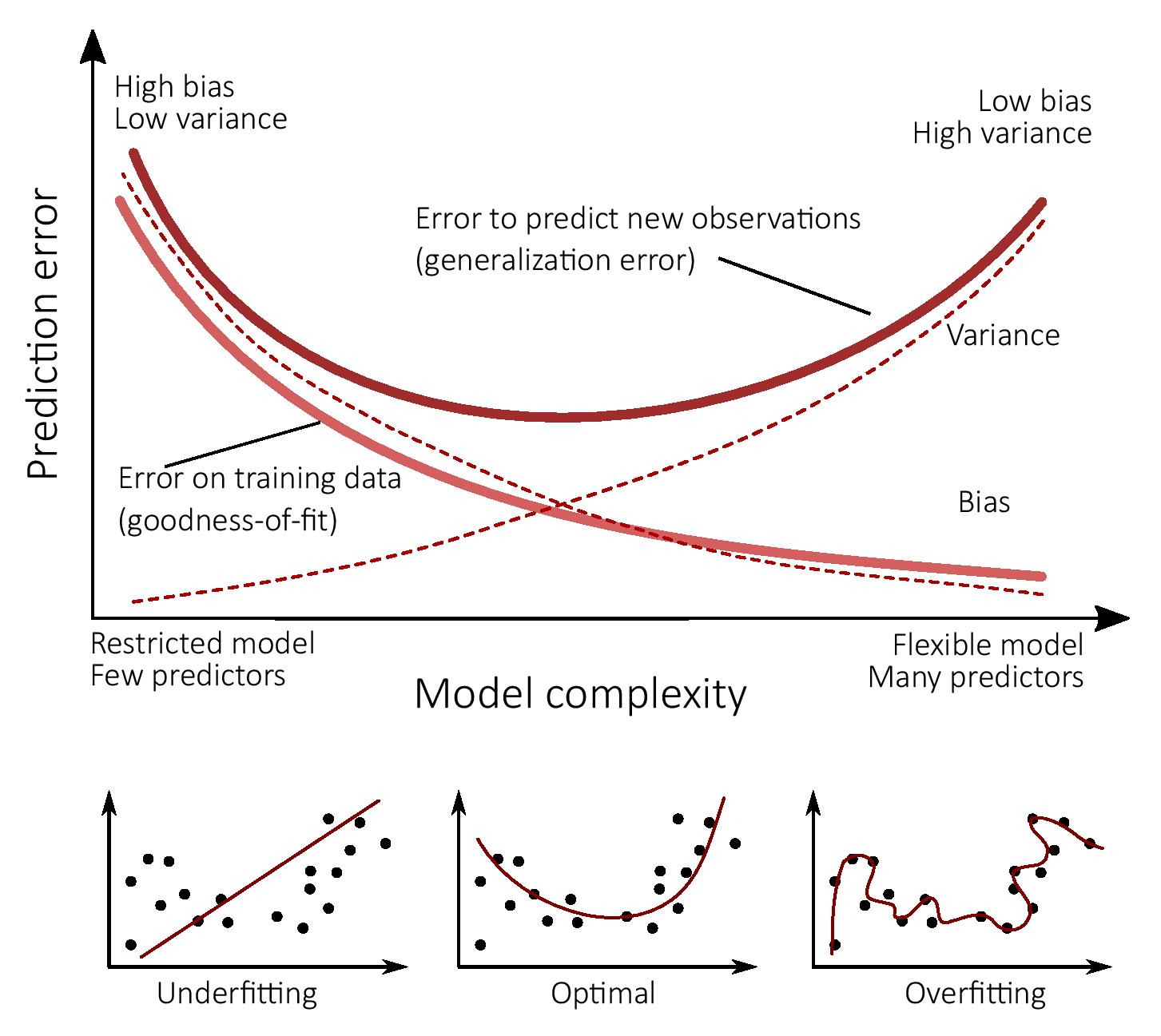
Bias-Variance trade-off

Expected validation MSE for a given value \(x_0\) can be decomposed into variance, squared bias and variance of the error \(\epsilon\) (unexplained variation):

\[ E(y_0 - \hat{f}(x_0))^2 = Var(\hat{f}(x_0)) + [Bias(\hat{f}(x_0))]^2 + Var(\epsilon) \]

Variance \(Var(\hat{f}(x_0))\)

How much \(\hat{f}\) would change if we estimated it using a different data set. High variance: small changes in the data result in large changes in \(\hat{f}\).

A high variance means that small changes in the calibration data lead to large changes in the model, which is in most cases undesirable. Wide spread ML approaches are able to find a good balance by allowing some flexibility in the model functional form, but at the same time reduce variance and thus not react to every small change in the data.

Bias \(Bias(\hat{f}(x_0))\)

Error that is introduced by approximating a real-world problem, which may be extremely complicated, by a much simpler model. E.g. linear regression assumes linearity which is unlikely to be the true model.

17.3 Common machine learning strategies

Successfull ML approaches find a good balance between bias and variance.

. . .

Different strategies for supervised learning, how this can be achieved:

Regularization Linear regression for large number of correlated predictors
Decision trees Step-wise splitting of data
Gradient boosting Forward selection
Bagging Fit and aggregate multiple models (often of the same type)
Support vector machines Estimate high-dimensional kernels
Artificial neural networks Transforming the data with a large number of weights

. . .

→ We will later focus on Bagging with decision trees (=Random Forest).

17.4 Regularization – problem

Problem

Select linear regression with stepwise forward/backward, best subset: Most often does not find true model, does overfit, selection is binary – a predictor is either in or out.
Correlated predictors cause problems in ordinary least squares regression.

Example

We want to predict yearly rainfall (mm) from elevation (m) and temperature (°C).

\(rainfall ~ = ~-912*temperature + 915*elevation\)

Elevation and temperature are strongly, negatively correlated, and might cause inflated coefficients that “cancel” each other out.

Regularization – how does it work?

Shrinkage, Regularization include a predictor, but with smaller, down-weighted coefficients.
Different approaches: Ridge regression, LASSO.
Minimize mean squared error as in “normal” regression plus a penalty for the size of the coefficients \(\beta\) (simplified):

\(\hat{\beta}_{lasso} = argmin \left\lbrace ~MSE + \lambda*| sum(\beta) | ~\right\rbrace\)

→ Useful when linear relationship present or needed and when predictors are numerous and correlated.

→ Performance often inferior compared to other methods.

17.5 Decision Trees

Recursive partitioning of predictor space → split by threshold, go on by dividing the new sub-regions
Results in simple, interpretable rules.
Single trees have high variance, small changes in the data change the trees often a lot.

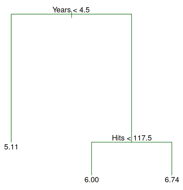
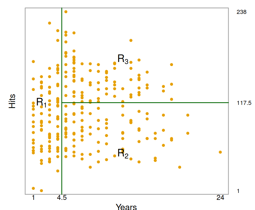
We use the Hitters data set to predict a baseball player’s Salary based on Years (the number of years that he has played in the major leagues) and Hits (the number of hits that he made in the previous year).

17.6 Gradient boosting

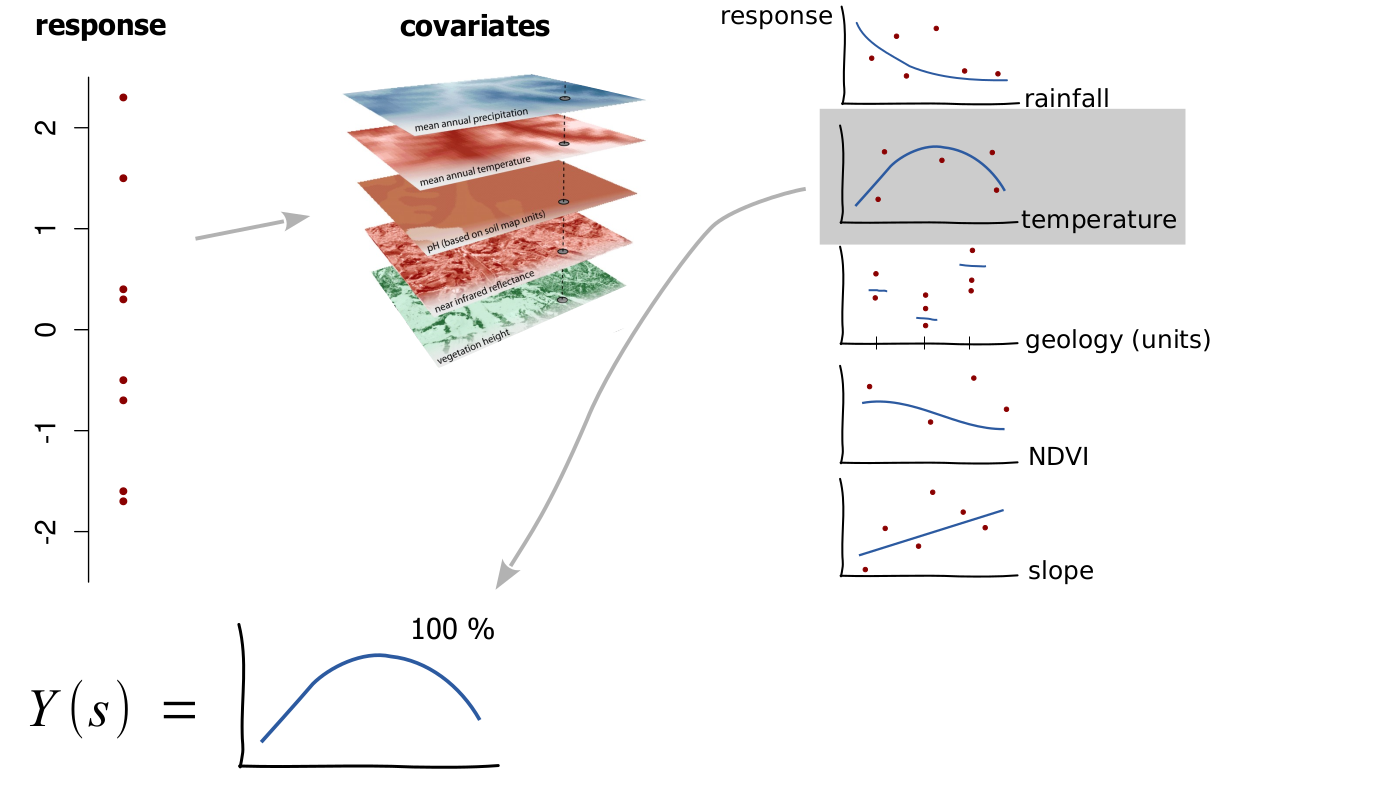
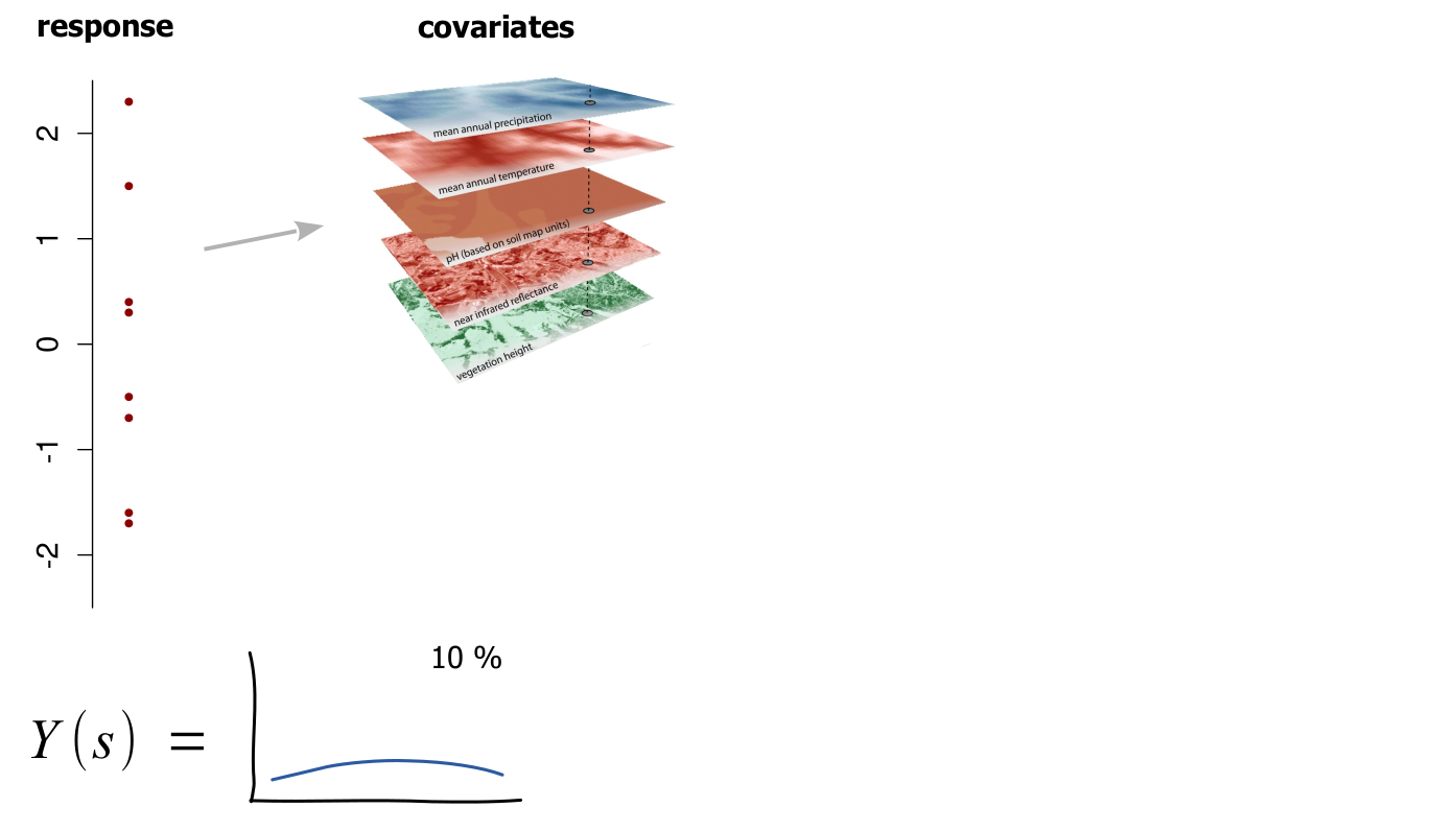
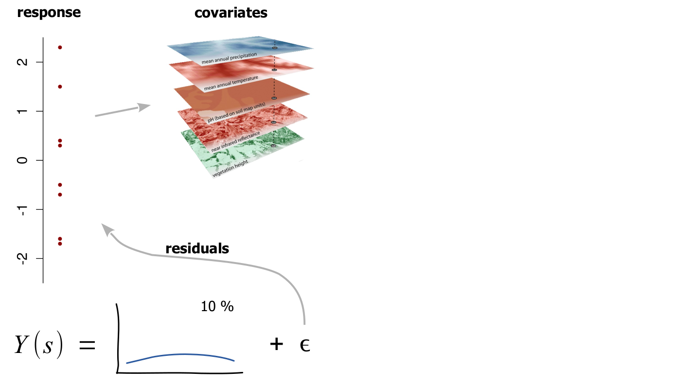
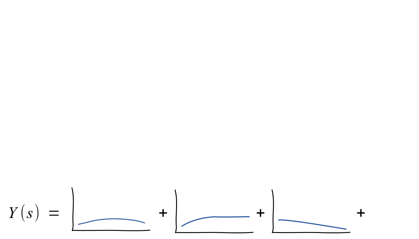
Smart forward selection that sequentially builds the model.
Baselearners: the functions that are added at each step.
At each step the baselearner is fit to the residuals of the previous step.
Baselearners can be: linear, smooth splines, spatial surfaces or short decision trees (most frequent).
Uses weak learners: the functions added in each step are down-weighted, model grows only slowly.

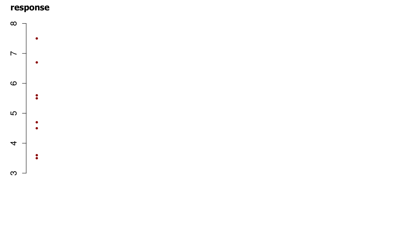
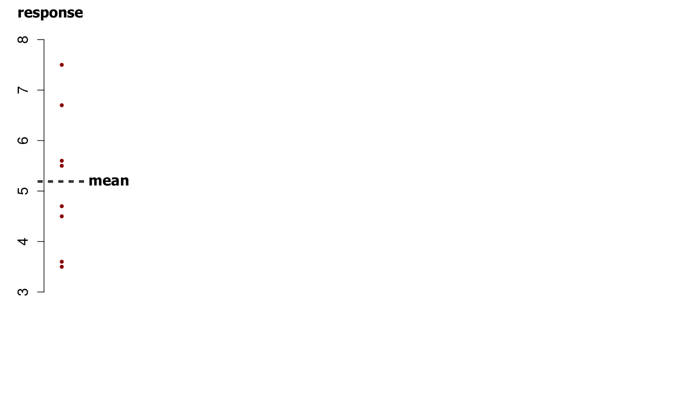
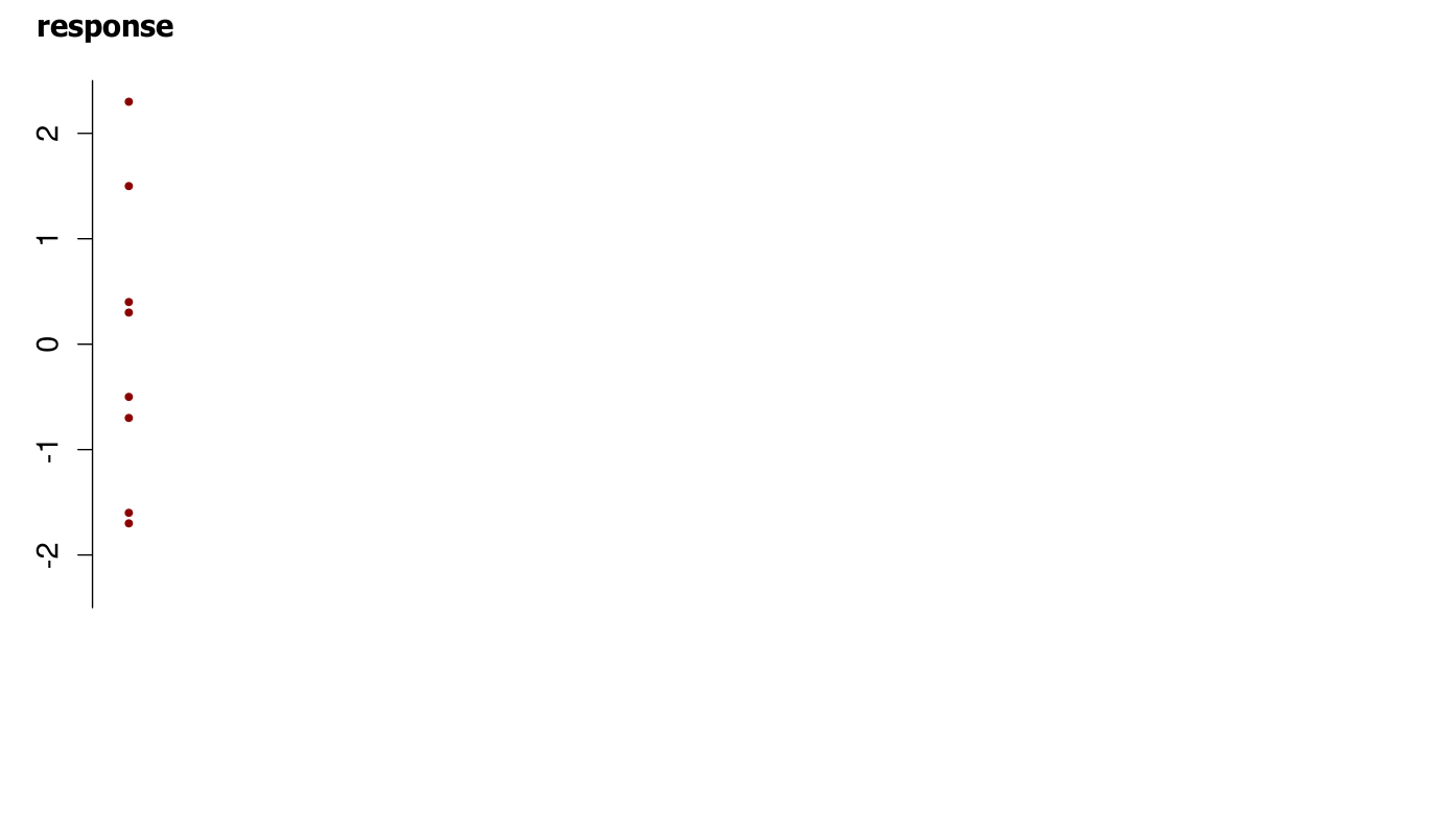
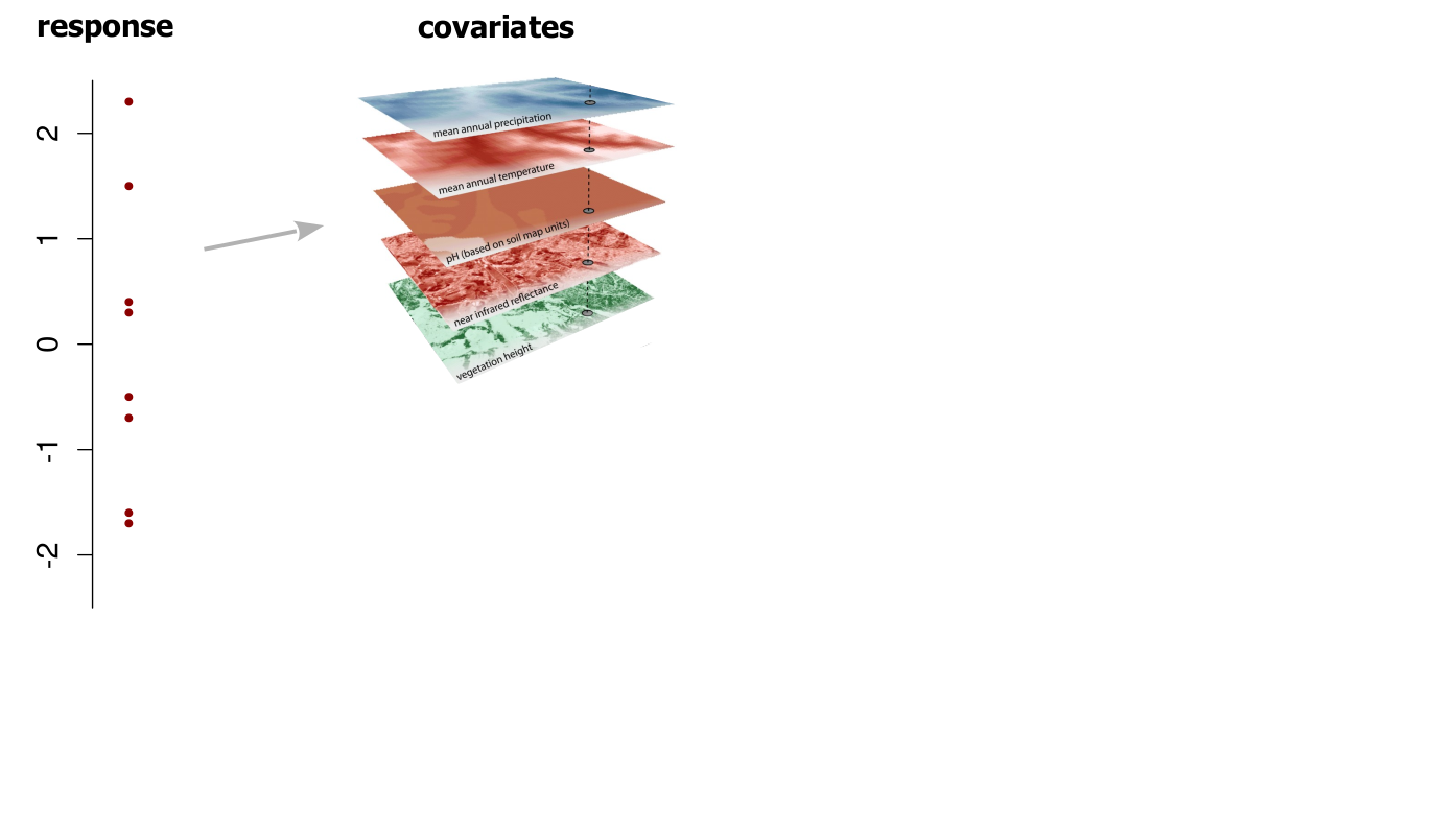
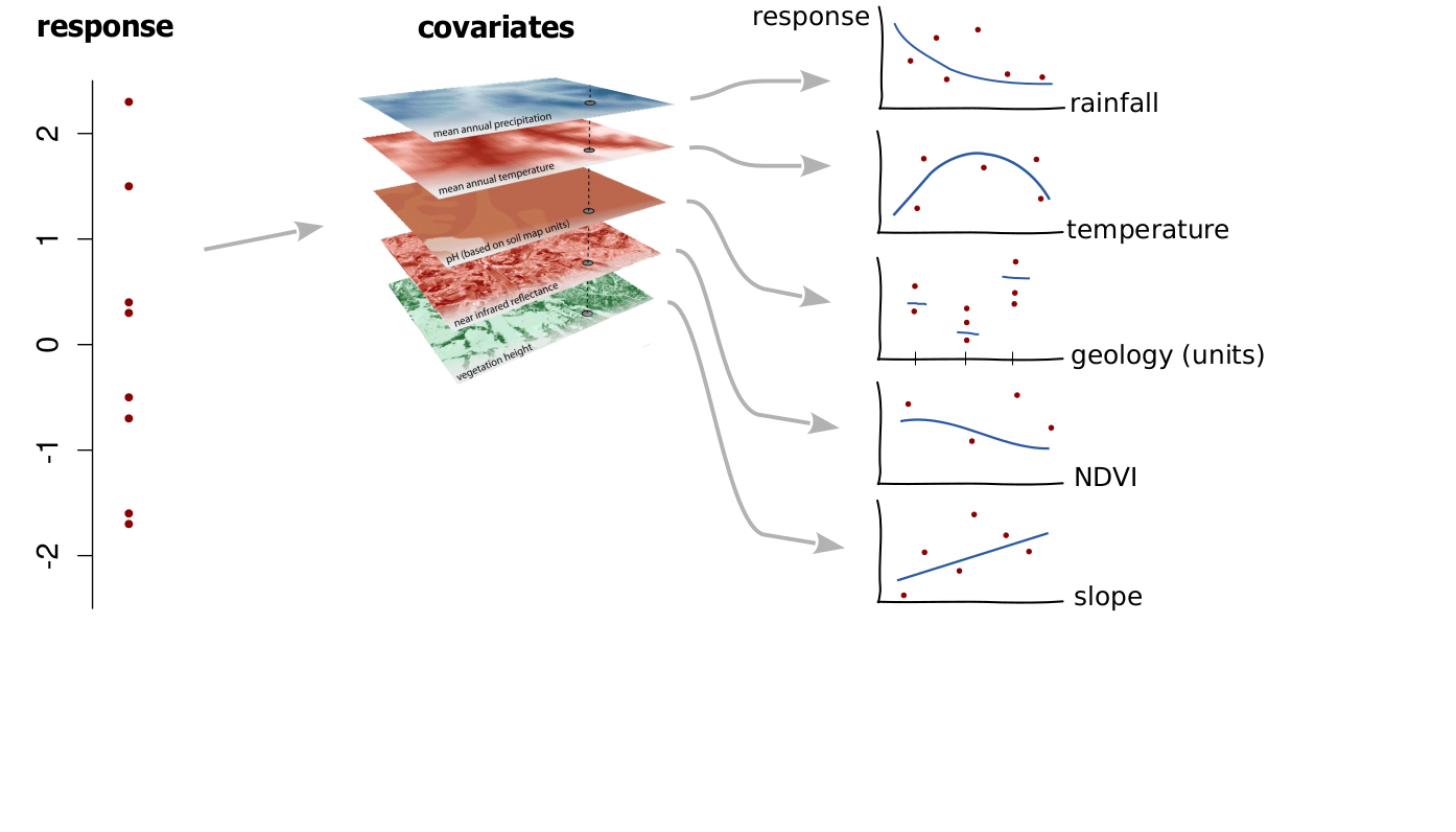
Gradient boosting – mini example

17.7 Bagging – bootstrap aggregation

Bagging = Bootstrap and aggregate
Bootstrap :
- Uniform resampling the data with replacement
- Draw a random set from your original data, some data points are selected 1, 2 or more times, about 30 % of the data is not selected
- Imitates multiple sampling campaigns (no change of response distribution)
Form e.g. 500 boostrap samples and fit model to each
Prediction = average of all predictions of those 500 models
Meaningful for low-bias, high-variance procedures

. . .

→ Most famous bagging algorithm: Random Forest bagging with additional trick to make trees non-similar (random predictor selection at each tree node split)

17.8 Support Vector Machines

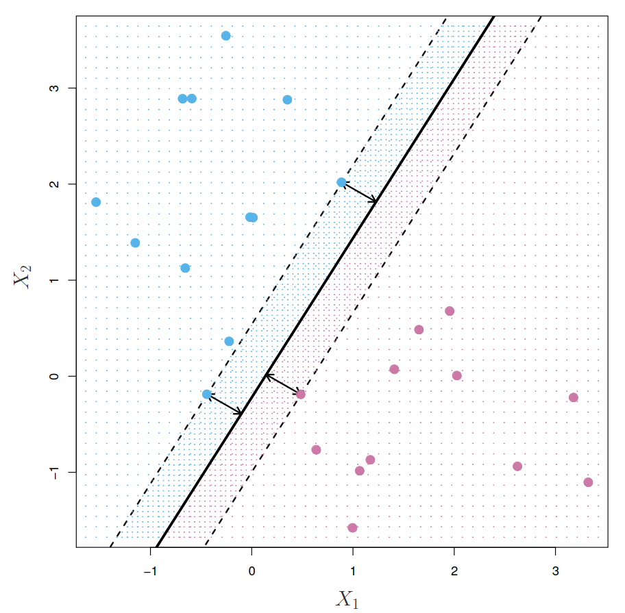
Find margin-maximizing hyperplane.
Nonlinear boundaries.
Effective for moderate-sized datasets.

Here illustrated for classification: split two classes as well as possible using values of \(X_1\) and \(X_2\).

Split data by a separating line (2 predictors) or separating plane (3 predictors) or hyperplane (>3 predictors) that is the farthest away from the observations.

The hyperplane is built up by support vectors (data points nearby the split).

Support vector machines – from linear to kernels

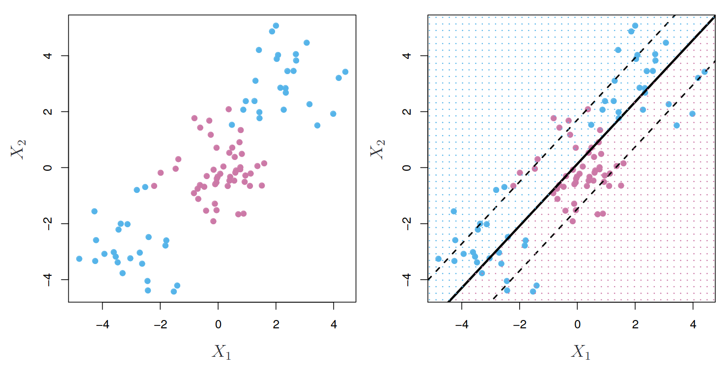
The observations fall into two classes, with a non-linear boundary between them.

The support vector classifier seeks a linear boundary, and consequently performs very poorly.

Support vector machines – from linear to kernels

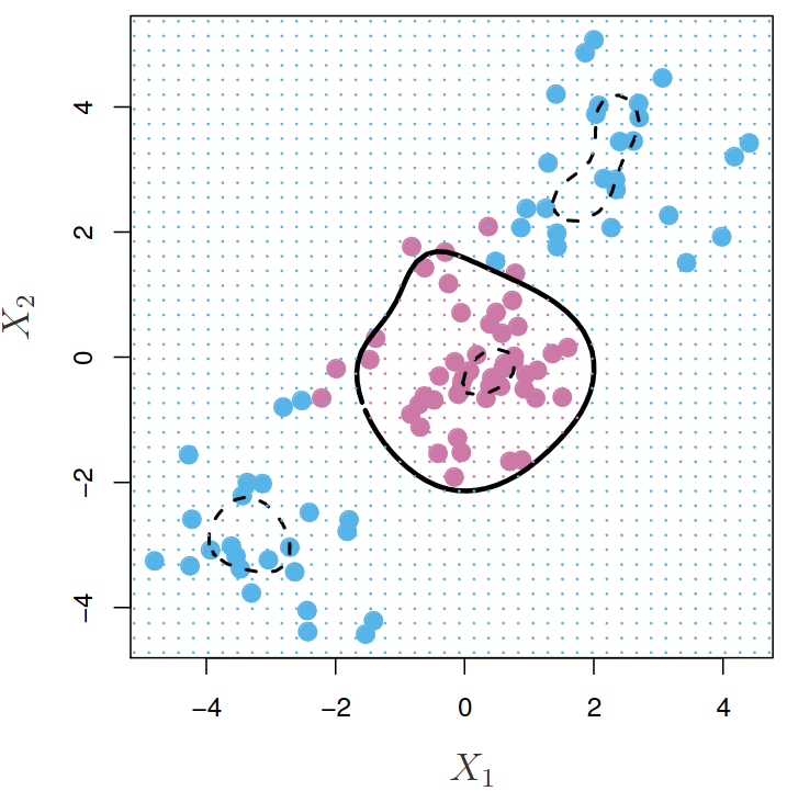
High-dimensional classifier.

Mainly depends on data points in the center of the distribution, hence is robust to outliers.

17.9 Artificial Neural Networks

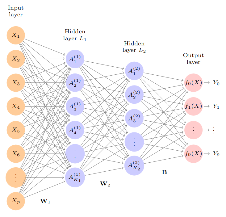
Layers of linear transformations (weights) + nonlinear activations (function to go from one layer to the next).
Architecture: setup of structure of those transformations.
Huge amount of weights need to be fitted.
Require large data, tuning + tweaking, computationaly demanding.

17.10 Which Strategy to Choose?

There is no free lunch in statistics!

We cannot know beforehand what works best with a new dataset.

. . .

Some thoughts & Practical Considerations

Keep it linear and simple → Regularization or Boosting with linear baselearners
Complex nonlinear patterns, threshold behavior → Tree-based methods like random forest or boosting with trees.
Highly correlated predictors → summarize with dimension reduction method.
Very large, complex data → neural networks.
Only small dataset → simpler models preferred.

Practical Considerations (continued)

Quality of data and availability of good predictors often matters more than algorithm choice.
Good model performance in literature for similar application, try this first.
No in-depth understanding of ML, better use method that is
- less sensitive to user choices like random forest (not neural networks),
- easier to implement (to avoid flaws).
Use a good validation strategy to assess model performance, if you want to compare multiple options.
Balance model performance, implementation effort, interpretability, and computation time.

17.11 Summary

Machine learning methods are algorithms that help us connect \(Y\) with \(X\) by searching for \(f(X)\).
A good balance between bias (“unflexible” model) and variance (“jumpy behavior”) has to be found.
Different options were introduced to balance bias and variance.
We need to select one (or more) of these options based on our situation (data, time, knowledge, computing facilities available).