library(sf)
library(compositions)
data(juraset)
d <- st_as_sf(juraset, coords = c("X", "Y"))
plot(d[3])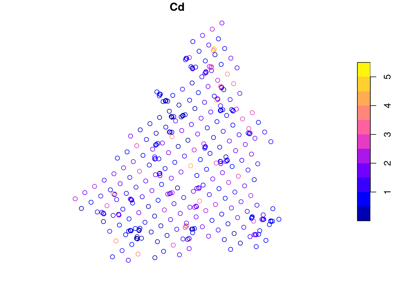
Download slides PDF
The PDF contains what was shown during the lecture. Some of these websites include additional text in light gray.
e-Lecture video
This lecture is available as recording.
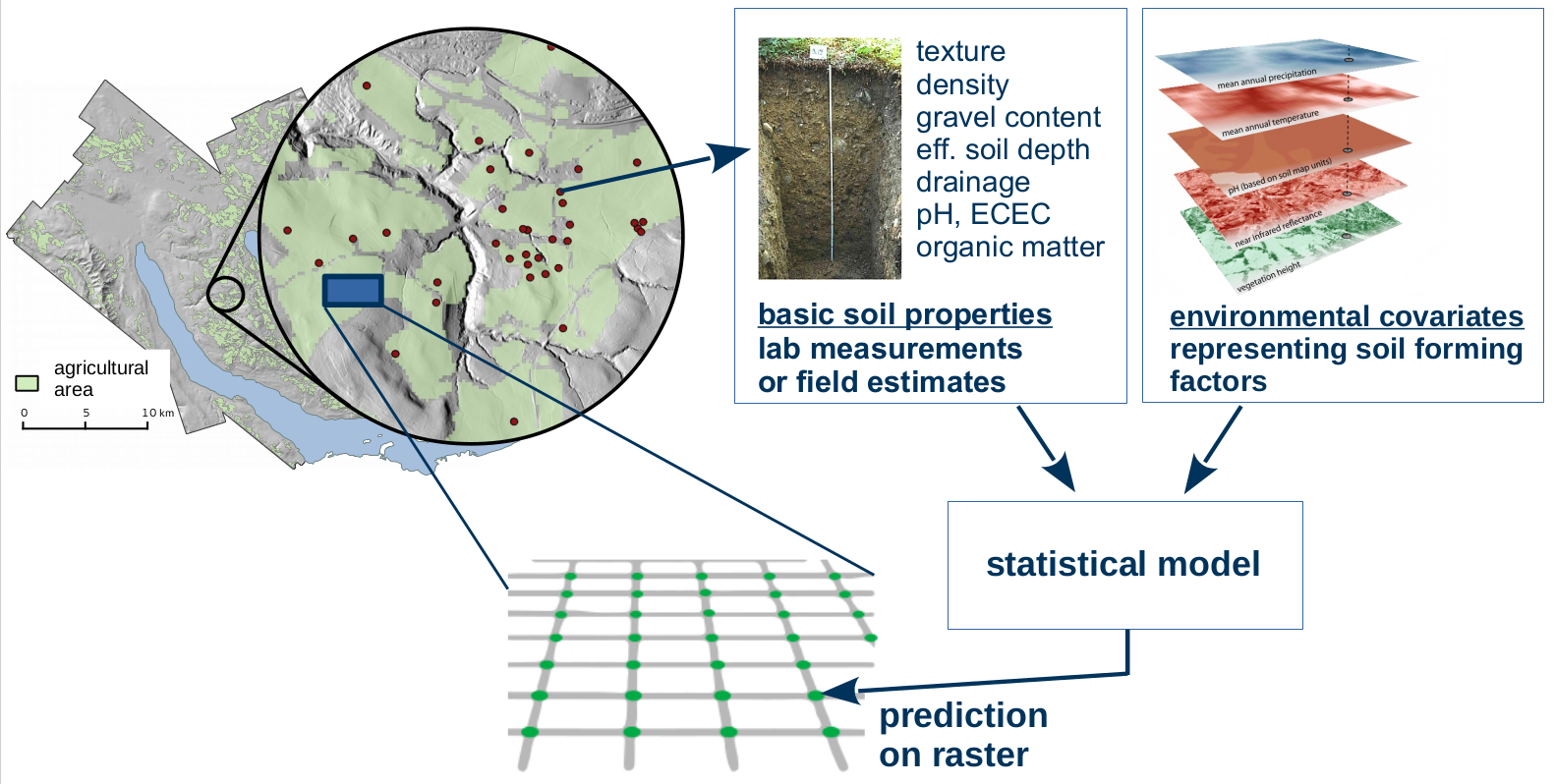
Spatial mapping: predicting or visualizing how a variable of interest varies across space.
Main goal: predict values at unsampled locations.
Point data (outcome, response, target variable)
Optional: Covariates (predictors, explanatory variables)
Prediction function
Spatial mapping links point data to raster covariates using a prediction function. Mapping can be done without raster covariates, then only the neighborhood relationships of the point data are used.
library(sf)
library(compositions)
data(juraset)
d <- st_as_sf(juraset, coords = c("X", "Y"))
plot(d[3])
library(gstat)
library(ggplot2)
no2 <- read.csv(system.file("external/no2.csv",package = "gstat"))
v.no2 <- st_as_sf(no2, crs = "OGC:CRS84", coords = c("station_longitude_deg", "station_latitude_deg"))
v.de <- read_sf("https://github.com/edzer/sdsr/raw/main/data/de_nuts1.gpkg")
ggplot() + geom_sf(data = v.de) + geom_sf(data = v.no2, mapping = aes(col = NO2)) 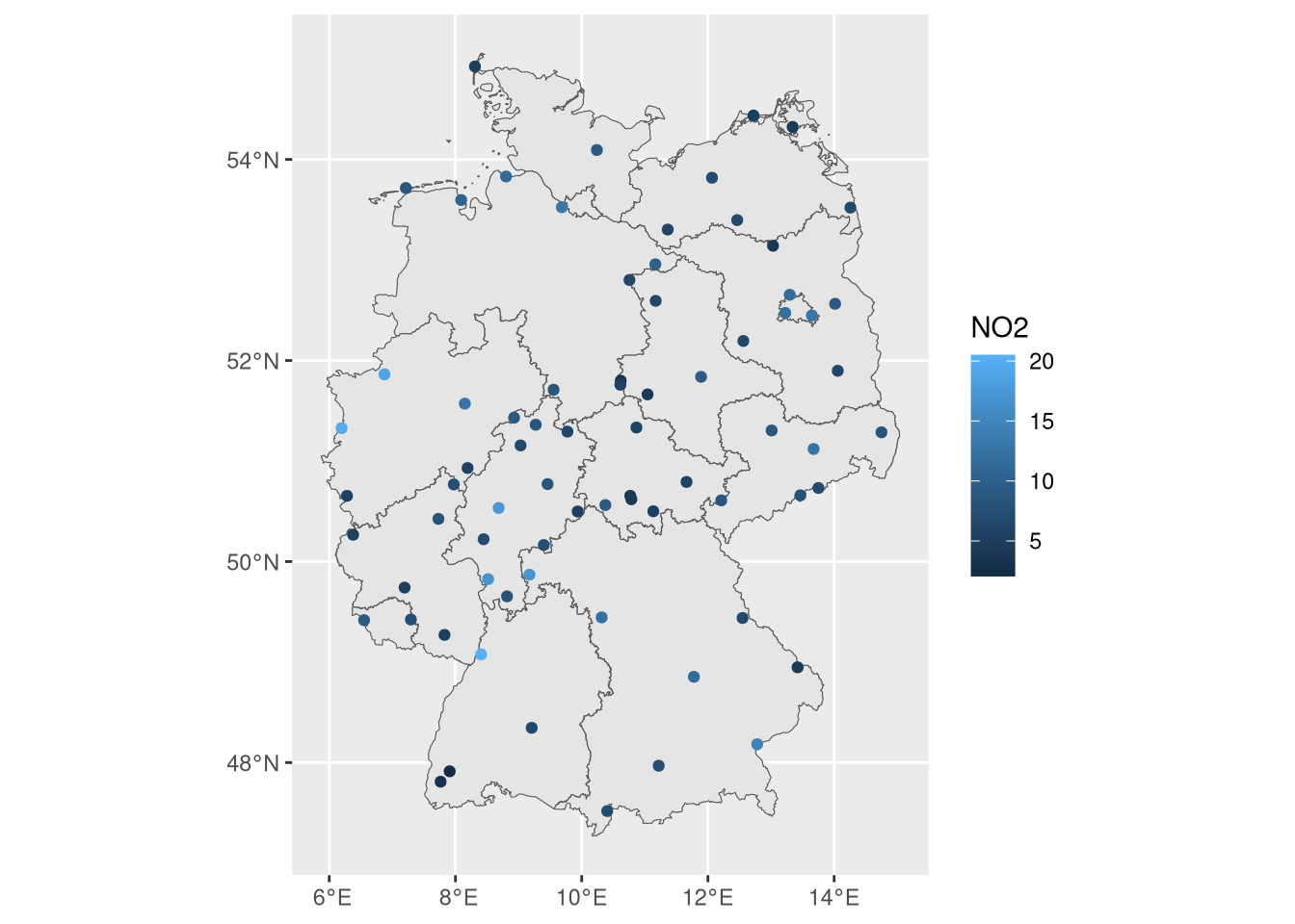
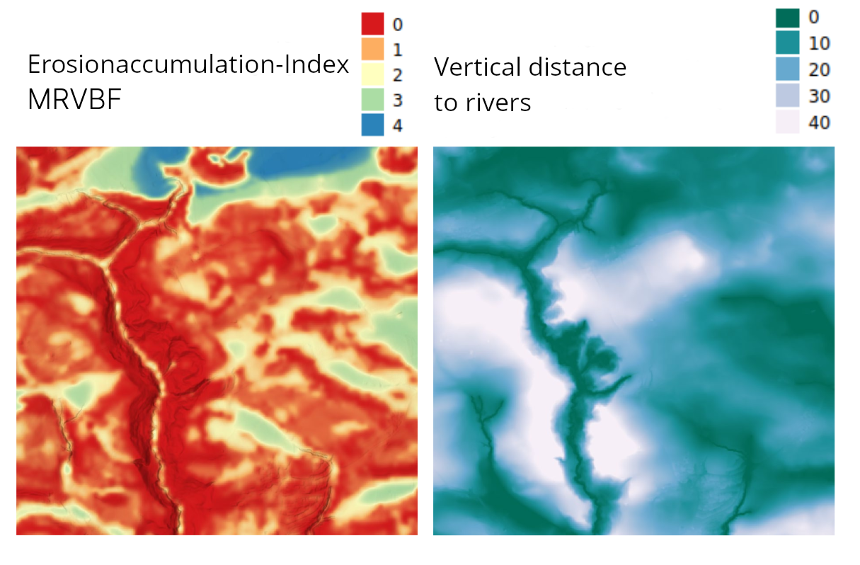
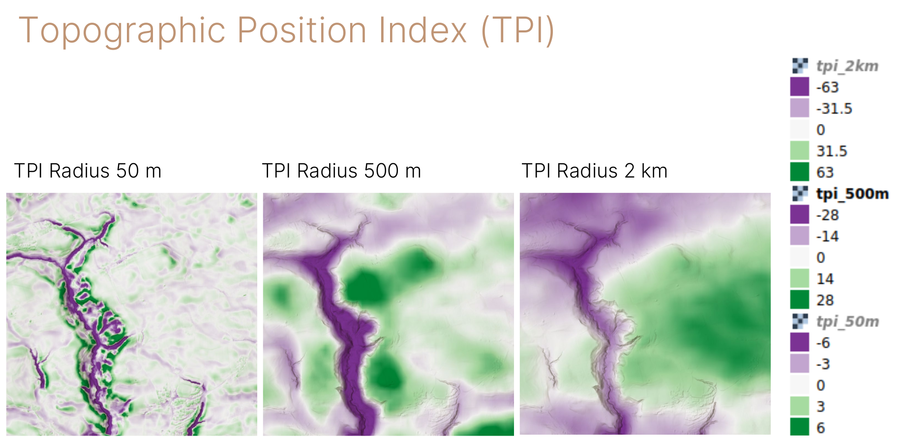
These are now just derivatives from one data set (elevation model). We could also have different datasets, and not be sure which is best to include. An example is meteorological data, where often different versions exist (e.g. average yearly rainfall over different periods, computed by different models or based on a different set of rainfall stations).
Also areal or lattice data can be possible predictors. Spatial distribution within areas is unknown and we have crisp boundaries, reflecting large uncertainty in the spatial allocation of the data.
A practical approach: transform to raster and apply smoothing.
library(sf)
library(mapview)
mapviewOptions(basemaps = "OpenStreetMap")
d <- st_read(system.file("shape/nc.shp", package = "sf"), quiet = TRUE)
mapview(d, zcol = "SID79")
Number of sudden infant deaths per counties of North Carolina (USA) in 1979.
Two main branches:
\(Y = \mathbf{X}\beta + E + Z\)
where
\(Y\) : observed point data at location \(i\)
\(\mathbf{X}\beta\) : general trend, e.g. a linear regression with covariates \(\mathbf{X}\) (raster data)
\(E\) : small scale fluctuations, spatial autocorrelation specified by a variogram
\(Z\) : random error (e.g. measurement error, part we cannot explain with model)
→ Explicit model for:
Points closer to each other are more similar, than points further away.
→ Yields prediction uncertainty directly, many special cases solved.
→ Classical statistics, relies on e.g. normally distributed residuals.
→ Selecting a trend model is often challenging.
\(Y = f(\mathbf{X}) + Z~~\) or \(~~Y = f(\mathbf{X}, I) + Z~~\) or \(~~Y = f_i(\mathbf{X}) + Z\)
where
\(Y\) : observed point data at locations \(i\)
\(f(X)\) : complex function, established by an algorithm using covariates \(\mathbf{X}\)
\(I\) : location \(i\) of the data points
\(Z\) : random error (e.g. measurement error, part we cannot explain with model)
→ Uses non-spatial prediction approach, sometimes integrates spatial position somehow.
→ Easy to find a model, relaxed statistical assumptions.
→ Spatial autocorrelation is less explicitly handled, mostly ad-hoc.
→ Drawback for special cases (e.g. uncertainty for a mean prediction of a region)
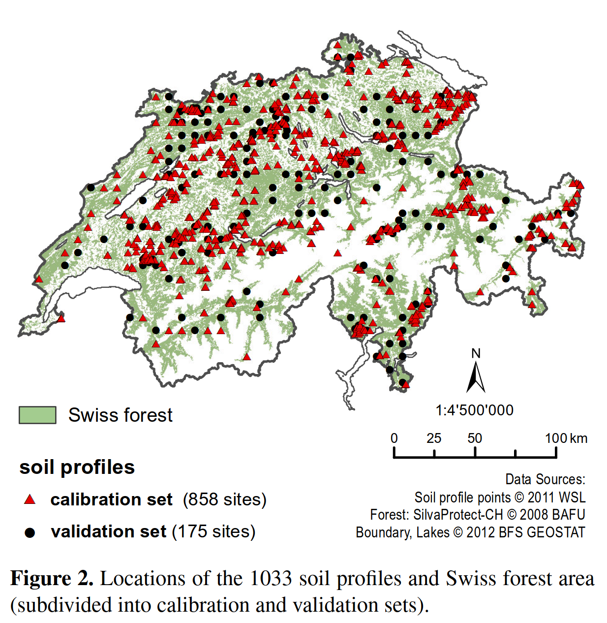
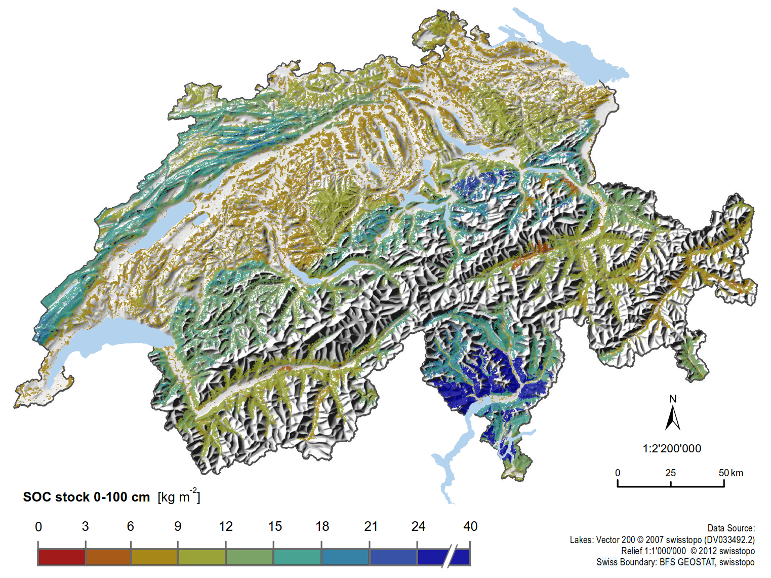
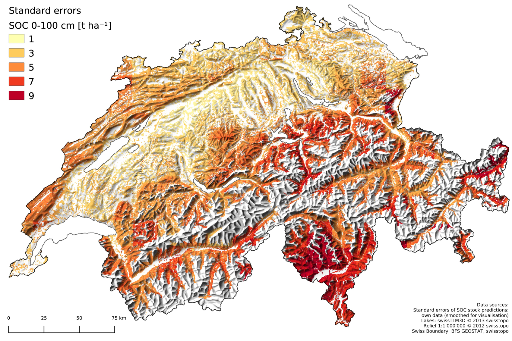
Swiss government needed data for greenhouse gas inventory.
→ Mapping of carbon stocks in forest soils using kriging with a linear trend model
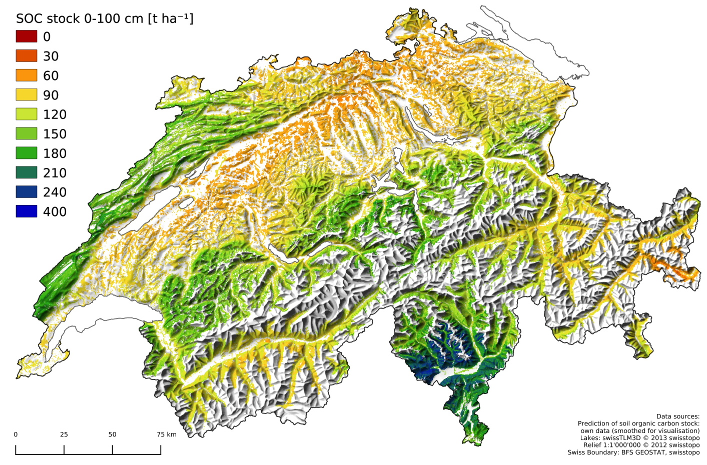
Some years later, 850 new soil point data became available.
→ Mapping with random forest
→ Point sampling is sparse & expensive.
→ End-users need actionable spatial information, not just point samples.
→ Supports decision-making, environmental assessment, resource or risk management.
Our objective is to
Compute spatial predictions of response variable for
Quantify uncertainty of these predictions,
Estimate relationships of spatial response variable and covariates.
In short, you will learn:
Handling spatial data in R
Find a prediction function / model
Investigate the spatial structure / auto-correlation of the data
Interpretation of the prediction model
Assess the performance of the predictions