library(georob)
library(mapview)
data(meuse)
coordinates(meuse) <- ~x+y
proj4string(meuse) <- CRS("+init=epsg:28992")
mapview(meuse, zcol = "zinc", map.types = "Esri.WorldImagery")15 Special cases in geostatistics
Download slides PDF
The PDF contains what was shown during the lecture. Some of these websites include additional text in light gray.
Geostatistical model: 2 special cases
There are many special cases for which the geostatitsical model has been expanded. Let’s have a look at two of them:
- 2 special cases to expand the geostatistical model
- lognormal kriging
- anisotropy
pro memoria: Model for Gaussian spatial data
Model for data: \(Y_{i} = S(\mathbf{x}_{i}) + Z_{i} = \mu(\mathbf{x}_{i}) + E(\mathbf{x}_{i}) + Z_{i}\)
with \(Y_{i}\): \(i^{\text{th}}\) datum; \(S(\mathbf{x}_{i})\): “signal” (true quantity) at location \(\mathbf{x}_{i}\); \(\mu(\mathbf{x}_{i})\): trend
\(\{E(\mathbf{x}_{i})\}\): a zero-mean Gaussian process, parametrized by covariance function \(\gamma(\mathbf{h}; \mathbf{\theta})\) or variogram \(V(\mathbf{h}; \mathbf{\theta})\)
\(Z_{i}\): iid Gaussian measurement error with variance \(\tau^2\)
Trend \(\mu(\mathbf{x}_{i})\) modeled by linear regression model with spatial covariates \(d_{k}(\mathbf{x}_{i})\)
\[ \mu(\mathbf{x}_{i}) = \sum_{k} d_{k}(\mathbf{x}_{i}) \beta_{k} = \mathbf{d}(\mathbf{x}_{i})^{T} \mathbf{\beta} \]
15.1 Lognormal universal kriging
Gaussian model fitted to log-transformed response variable \(Y(\mathbf{x}) = \log\big(U(\mathbf{x})\big)\)
(e.g. often pollution datasets)
⇒ Computing UK predictions for log-transformed response
⇒ How should we back-transform to original scale of response?
Lognormal distribution \[ Y = \log(U) \sim {\cal N}(\mu_{Y},\sigma_{Y}^2) \]
Expectation and variance of \(U\) \[ \begin{eqnarray*} \mathbb{E}[U] & = & \mu_{U} = \exp(\mu_{Y} + 0.5 \, \sigma_{Y}^2)\\ Var[U] & = & \mu_{U}^2 (\exp(\sigma_{Y}^2) -1 ) \end{eqnarray*} \]
Backtransformation for lognormal universal kriging
\(\exp\big(\hat{S}_{\mathrm{k}}(\mathbf{x}^\prime)\big)\) is a biased predictor of \(U(\mathbf{x}^\prime)\)
Unbiased back-transformation \[
\hat{U}_{\mathrm{lk}}(\mathbf{x}^\prime) = \exp
\left(\hat{S}_{\mathrm{k}}(\mathbf{x}^\prime)+0.5\left\{Var[S(\mathbf{x}^\prime)]
- Var[\hat{S}_{\mathrm{k}}(\mathbf{x}^\prime)]\right\}\right)
\]
Limits of prediction intervals can be back-transformed directly by \(\exp()\).
Back-transformation implemented in function lgnpp of R package georob.
Example: Lognormal UK Meuse zinc data
Example Meuse zn: Response distribution
par(mfrow=c(1,2))
hist(meuse@data$zinc, breaks = 20)
hist(log(meuse@data$zinc), breaks = 20)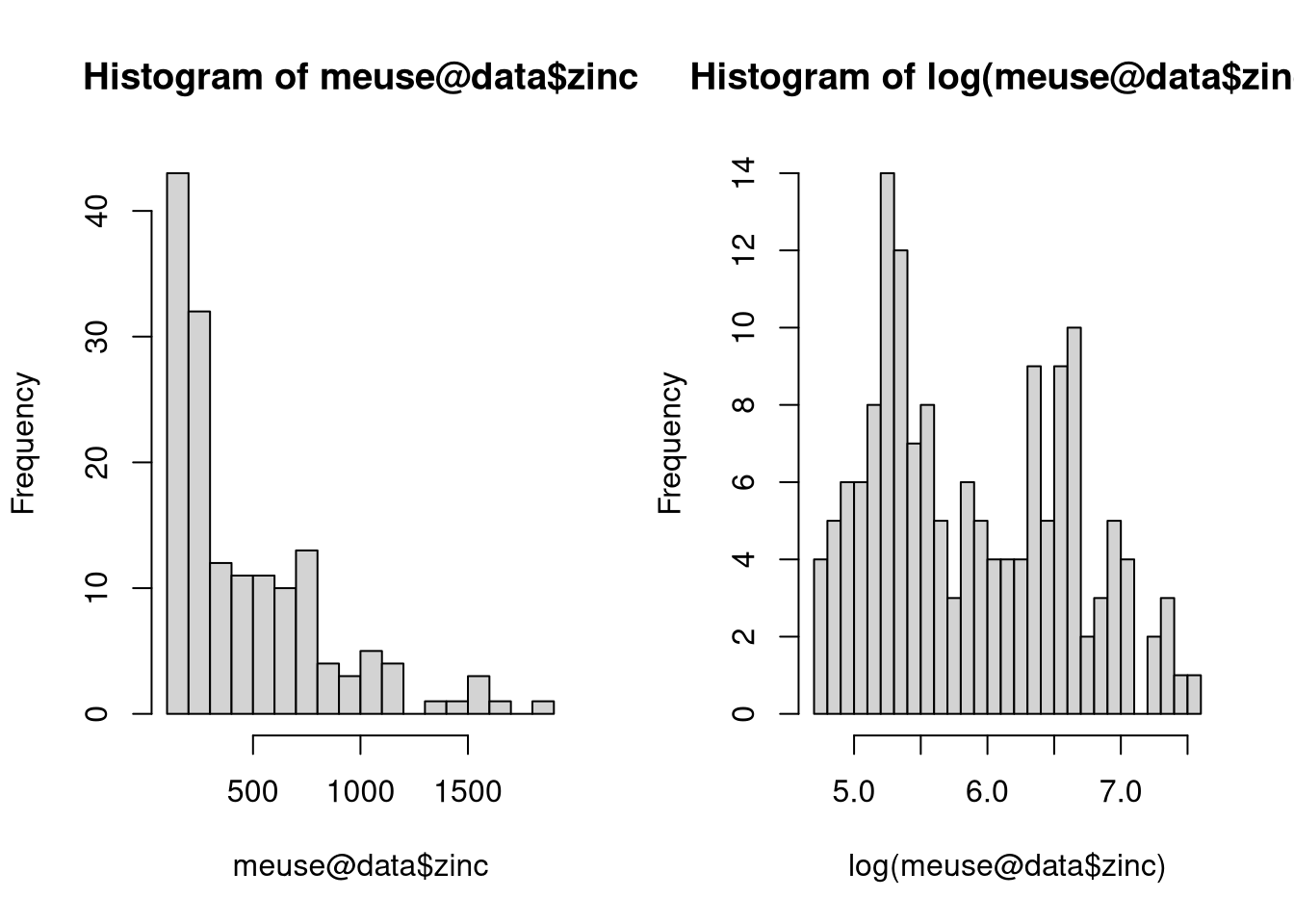
Example Meuse zn: OLS residuals
par(mfrow = c(1,2))
plot(lm(zinc ~ dist, meuse), 2)
plot(lm(log(zinc) ~ dist, meuse), 2)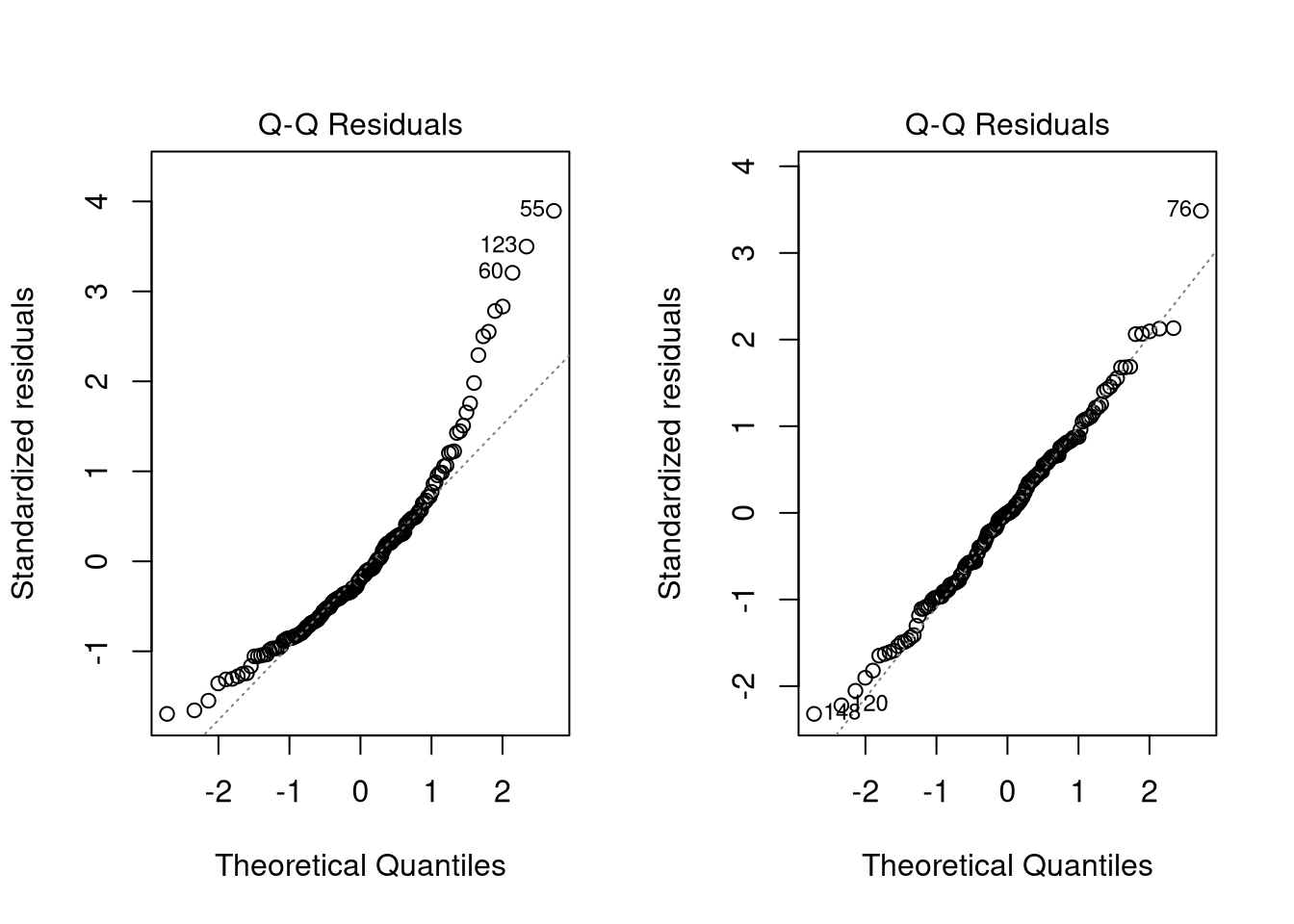
Example Meuse zn: REML fit
r.logzn <- georob(log(zinc)~sqrt(dist), meuse, locations=~x+y,
                  variogram.model="RMexp",
                  param=c(variance=0.15, nugget=0.05, scale=200),
                  tuning.psi=1000, control=control.georob(
                    cov.bhat=TRUE, cov.bhat.betahat=TRUE))
r.logzn
Tuning constant:  1000

Fixed effects coefficients:
(Intercept)   sqrt(dist)
      6.985       -2.567

Variogram:  RMexp
        variance    snugget(fixed)            nugget             scale
         0.14910           0.00000           0.04867         192.52854
Example Meuse zn: REML variogram
plot(r.logzn, lag.dist.def=60, max.lag=1500)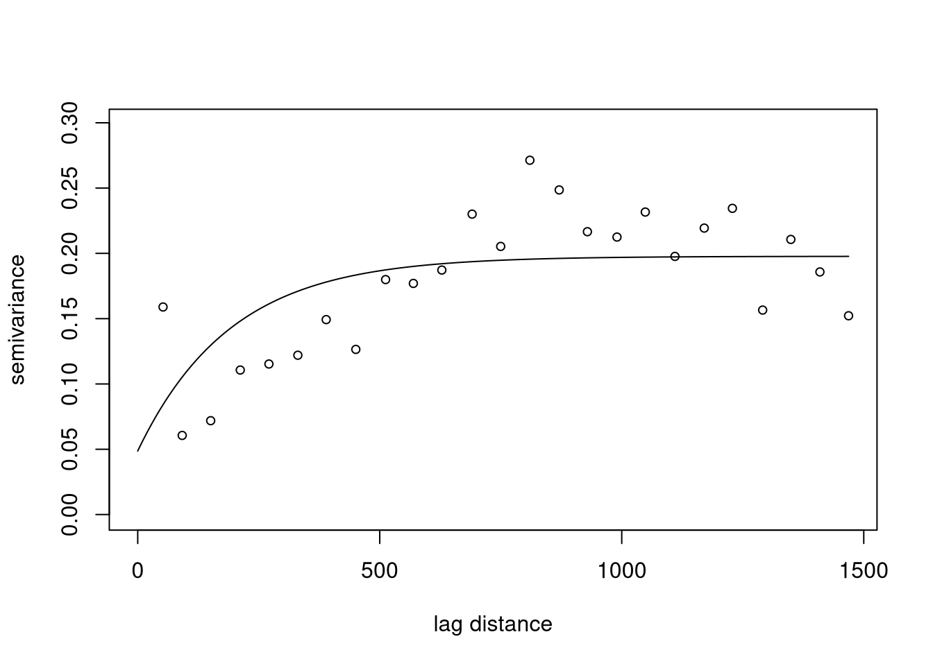
Example Meuse zn: Universal kriging prediction
data(meuse.grid)
coordinates(meuse.grid) <- ~x+y
gridded(meuse.grid) <- TRUE
r.luk <- predict(r.logzn, newdata=meuse.grid,
  control=control.predict.georob(extended.output=TRUE))
str(r.luk@data)
'data.frame': 3103 obs. of 8 variables:
$ pred : num 7.03 7.05 6.75 6.49 7.07 ...
$ se : num 0.362 0.335 0.342 0.349 0.288 ...
$ lower : num 6.32 6.39 6.08 5.8 6.5 ...
$ upper : num 7.73 7.7 7.42 7.17 7.63 ...
$ trend : num 6.99 6.99 6.7 6.45 6.99 ...
$ var.pred : num 0.0388 0.0539 0.0437 0.0357 0.0787 ...
$ cov.pred.target: num 0.0285 0.0453 0.0379 0.0315 0.0724 ...
$ var.target : num 0.149 0.149 0.149 0.149 0.149 ...
- attr(*, "variogram.object")=List of 1
..$ :List of 9
.. ..$ variogram.model: chr "RMexp"
.. ..$ param : Named num [1:4] 0.1491 0 0.0487 192.5285
.. .. ..- attr(*, "names")= chr [1:4] "variance" "snugget" "nugget" "scale"
.. ..$ fit.param : Named logi [1:4] TRUE FALSE TRUE TRUE
.. .. ..- attr(*, "names")= chr [1:4] "variance" "snugget" "nugget" "scale"
.. ..$ isotropic : logi TRUE
.. ..$ aniso : Named num [1:5] 1 1 90 90 0
.. .. ..- attr(*, "names")= chr [1:5] "f1" "f2" "omega" "phi" ...
.. ..$ fit.aniso : Named logi [1:5] FALSE FALSE FALSE FALSE FALSE
.. .. ..- attr(*, "names")= chr [1:5] "f1" "f2" "omega" "phi" ...
.. ..$ sincos :List of 6
.. .. ..$ co: num 6.12e-17
.. .. ..$ so: num 1
.. .. ..$ cp: num 6.12e-17
.. .. ..$ sp: num 1
.. .. ..$ cz: num 1
.. .. ..$ sz: num 0
.. ..$ rotmat : num [1:2, 1:2] 1.00 -6.12e-17 6.12e-17 1.00
.. ..$ sclmat : Named num [1:2] 1 1
.. .. ..- attr(*, "names")= chr [1:2] "" "f1"
- attr(*, "psi.func")= chr "logistic"
- attr(*, "tuning.psi")= num 1000
- attr(*, "type")= chr "signal"Example Meuse zn: Unbiased backtransformation
r.luk <- lgnpp(r.luk)
str(r.luk@data)
'data.frame': 3103 obs. of 12 variables:
$ pred : num 7.03 7.05 6.75 6.49 7.07 ...
$ se : num 0.362 0.335 0.342 0.349 0.288 ...
$ lower : num 6.32 6.39 6.08 5.8 6.5 ...
$ upper : num 7.73 7.7 7.42 7.17 7.63 ...
$ trend : num 6.99 6.99 6.7 6.45 6.99 ...
$ var.pred : num 0.0388 0.0539 0.0437 0.0357 0.0787 ...
$ cov.pred.target: num 0.0285 0.0453 0.0379 0.0315 0.0724 ...
$ var.target : num 0.149 0.149 0.149 0.149 0.149 ...
$ lgn.pred : num 1189 1204 902 694 1215 ...
$ lgn.se : num 440 409 314 249 354 ...
$ lgn.lower : num 554 595 438 331 667 ...
$ lgn.upper : num 2286 2215 1673 1299 2064 ...
- attr(*, "variogram.object")=List of 1
..$ :List of 9
.. ..$ variogram.model: chr "RMexp"
.. ..$ param : Named num [1:4] 0.1491 0 0.0487 192.5285
.. .. ..- attr(*, "names")= chr [1:4] "variance" "snugget" "nugget" "scale"
.. ..$ fit.param : Named logi [1:4] TRUE FALSE TRUE TRUE
.. .. ..- attr(*, "names")= chr [1:4] "variance" "snugget" "nugget" "scale"
.. ..$ isotropic : logi TRUE
.. ..$ aniso : Named num [1:5] 1 1 90 90 0
.. .. ..- attr(*, "names")= chr [1:5] "f1" "f2" "omega" "phi" ...
.. ..$ fit.aniso : Named logi [1:5] FALSE FALSE FALSE FALSE FALSE
.. .. ..- attr(*, "names")= chr [1:5] "f1" "f2" "omega" "phi" ...
.. ..$ sincos :List of 6
.. .. ..$ co: num 6.12e-17
.. .. ..$ so: num 1
.. .. ..$ cp: num 6.12e-17
.. .. ..$ sp: num 1
.. .. ..$ cz: num 1
.. .. ..$ sz: num 0
.. ..$ rotmat : num [1:2, 1:2] 1.00 -6.12e-17 6.12e-17 1.00
.. ..$ sclmat : Named num [1:2] 1 1
.. .. ..- attr(*, "names")= chr [1:2] "" "f1"
- attr(*, "type")= chr "signal"Example Meuse zn: Predicted maps
library(terra)
r.luk <- rast(r.luk)
par(mfrow=c(1,2))
plot(r.luk["^pred$"], main = "UK prediction log(zn)")
plot(r.luk["lgn.pred"], main = "LUK prediction zn")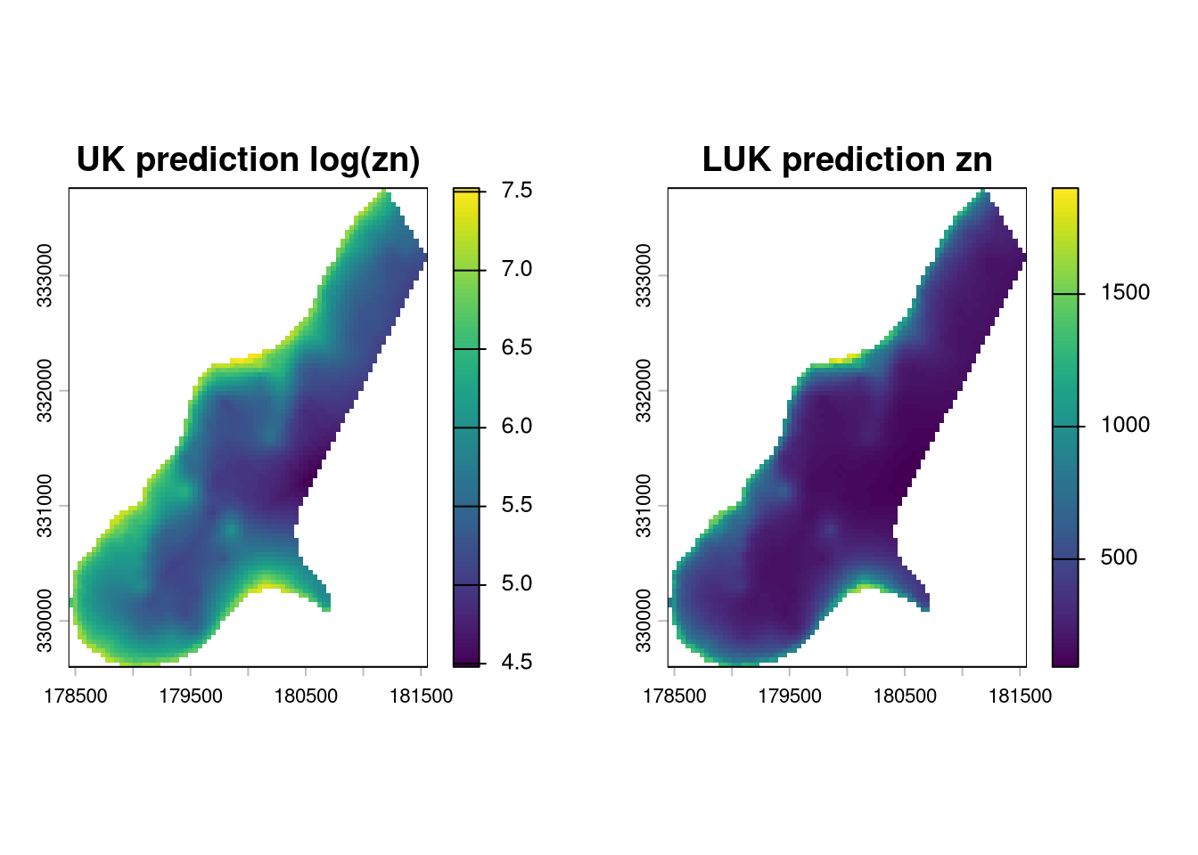
Example Meuse zn: Predicted standard errors
par(mfrow=c(1,2))
plot(r.luk["^se$"], main = "UK standard error log(zn)")
plot(r.luk["lgn.se"], main = "LUK stanard error zn")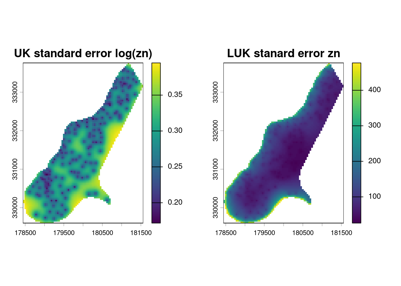
15.2 Anisotropic variograms
Spatial auto-correlation can vary from one direction to the other, i.e. it can be anisotropic.
In many instances the anisotropy is such that it could be made isotropic by a simple linear transformation of the spatial coordinates. ⇒ geometrically anisotropic variogram function
Idea: rotate and stretch/shrink components of \(\mathbf{x}\) such that the stochastic process is isotropic in the transformed coordinate system
\[ V(h^*) = V\left( \sqrt{(\mathbf{h}\mathbf{A})^\mathrm{T}\mathbf{A}\mathbf{h}} \right) \]
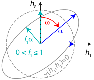
Iso-semivariances contours are ellipsoids in space of non-transformed coordinates and are mapped by transformation:
\[ \mathbf{A} = \left[\begin{array}{cc} 1/\alpha & 0\\ 0 & 1/(f_{1}\alpha) \end{array}\right] \left[\begin{array}{cc} \cos(\omega) & \sin(\omega) \\ -\sin(\omega) & \cos(\omega) \end{array}\right] \]
Example: elevation data
data(elevation, package="georob")
d.elevation <- elevation
d.elevation$res <- residuals(lm(height~y, d.elevation))
plot(y~x, d.elevation, cex=sqrt(abs(res)), asp=1,
  col=c("blue", NA, "orange")[sign(res)+2])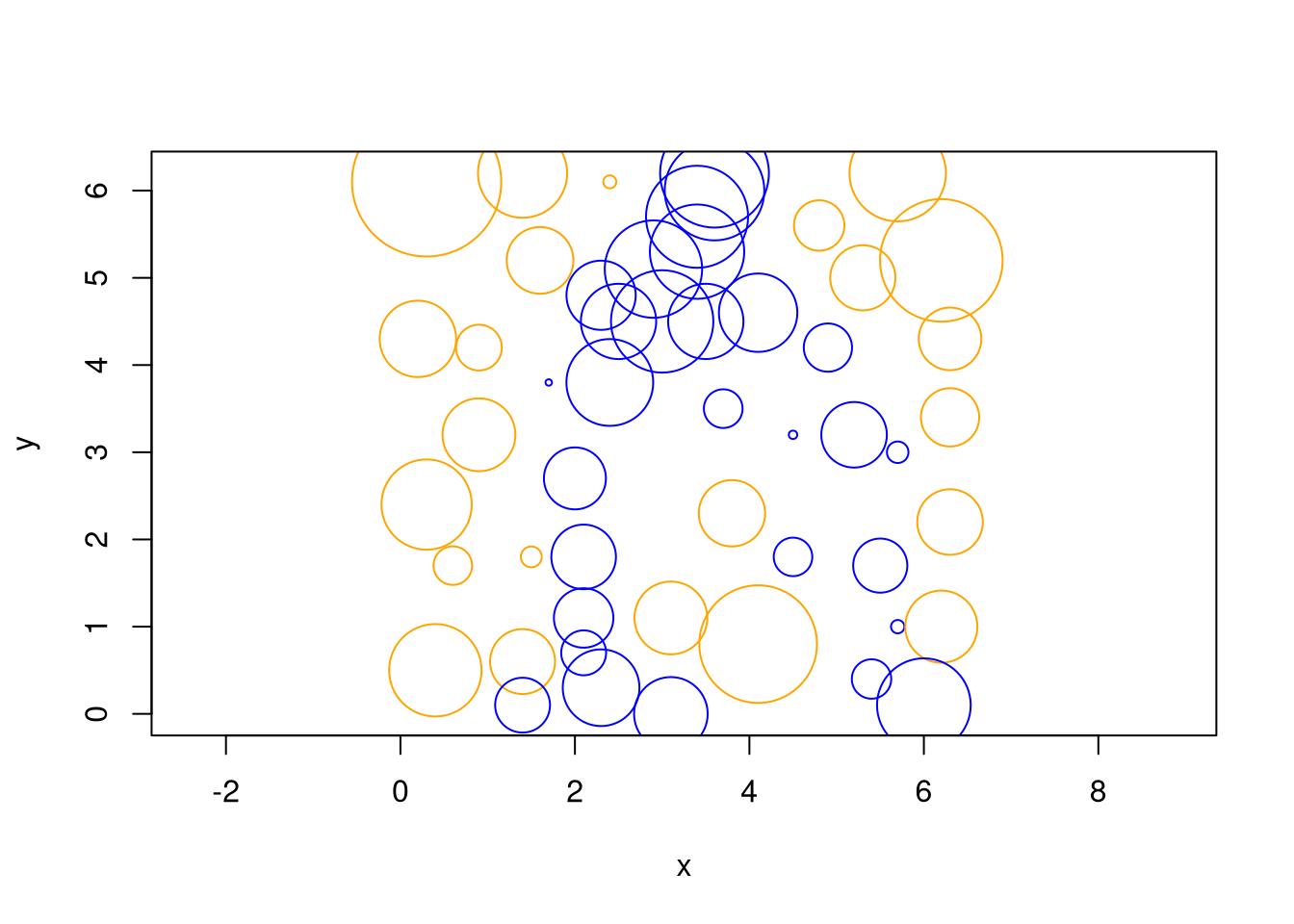
Example: elevation data - directional sample variogram
r.sv <- sample.variogram(d.elevation$res,
  locations=as.matrix(d.elevation[, c("x","y")]),
  lag.dist.def=0.5, xy.angle.def=c(0, 45, 135, 180))
summary(r.sv)
Sample variogram estimator: qn

Summary of lag distances
   Min. 1st Qu.  Median    Mean 3rd Qu.    Max.
 0.3812  2.2244  4.2278  4.1295  6.1756  8.2759

Summary of number of pairs per lag and distance classes
   Min. 1st Qu.  Median    Mean 3rd Qu.    Max.
   1.00   11.00   45.00   40.18   63.00   73.00

Angle classes in xy-plane: (-45,45] (45,135]
Angle classes in xz-plane: [0,180]
Example: elevation data - directional sample variogram
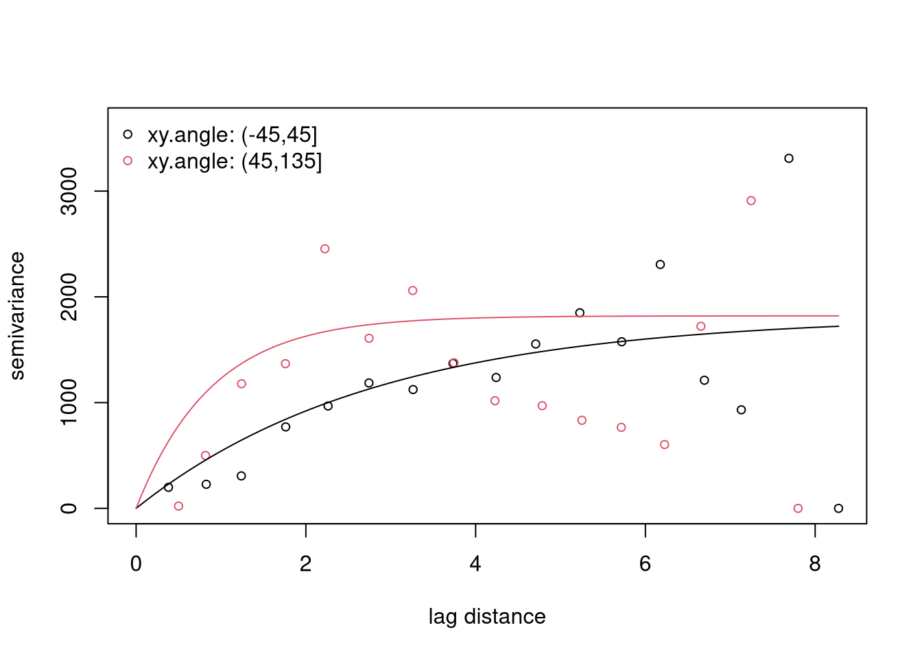
plot(r.sv)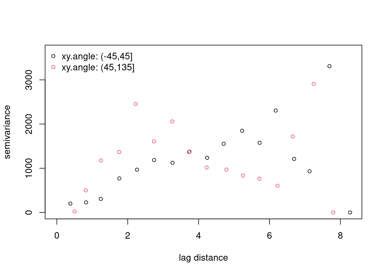
Example: elevation data - fitted directional variogram
r.exp <- fit.variogram.model(r.sv,
  variogram.model="RMexp",
  param=c(variance=1500, nugget=10, scale=4),
  aniso = default.aniso(f1 = 0.4, omega = 0),
  fit.aniso = default.fit.aniso(f1 = TRUE, omega = TRUE))
r.exp
Variogram:  RMexp
        variance    snugget(fixed)            nugget             scale
       1.820e+03         0.000e+00         1.289e-07         1.256e+02

              f1         f2(fixed)             omega        phi(fixed)
        0.006757          1.000000         17.415945         90.000000
     zeta(fixed)
        0.000000
Example: elevation data - fitted directional variogram
plot(r.sv)
lines(r.exp, xy.angle=c(0, 90))