6 Theory: Stochastic process
Download slides PDF
The PDF contains what was shown during the lecture. Some of these websites include additional text in light gray.
Overview
Chapters 6-12
Geostatistics: theory, variogram properties, maximum likelihood, prediction
Stochastic process
Realization of stochastic process
Variogram functions
Sample variogram and fitting of variogram function
Maximum likelihood estimation of model parameters
Model selection/inference
Predictions for ordinary and universal/external drift kriging
6.1 Stochastic process
Terminology and model notation (chapter 4)
Model for data: \(Y_{i} = S(\mathbf{x}_{i}) + Z_{i}\)
where
\(Y_{i}\) : \(i^\mathrm{th}\) datum
\(S(\mathbf{x}_{i})\) : “signal” (= true quantity) at location \(\mathbf{x}_{i}\)
\(Z_{i}\) : iid. random measurement error
Decomposition of signal into trend \(\mu(\mathbf{x}_{i})\) and stochastic fluctuation:
\[ S(\mathbf{x}_{i}) = \mu(\mathbf{x}_{i}) + E(\mathbf{x}_{i}) \]
where commonly a linear model is used for \(\mu(\mathbf{x}_{i})\)
\[ \mu(\mathbf{x}_{i}) = \sum_{k} d_{k}(\mathbf{x}_{i}) \beta_{k} = \mathbf{d}(\mathbf{x}_{i})^\mathrm{T} \mathbf{\beta} \] with \(d_{k}(\mathbf{x}_{i})\) denoting (spatial) covariates and \(\{E(\mathbf{x}_{i})\}\) a zero mean stochastic process (random field).
Realization of stochastic process
Spatial phenomena obey laws of physics ⇒ are deterministic, have physical causes
Numerous processes and interactions thereof produce current complex outcome
Variation appears random ⇒ in geostatistical terms viewed as a random process
e.g. rainfall pattern, soil properties, air pollution as a realization of a random process
Each location \(x\) is associated with a suite of values with a known distribution
Actual value observed at \(x\) is viewed as one value of this distribution, allocated at random
Random function has no mathematical description, but “structure” in the sense of correlation in space (or time) and describes relation of random values at different locations to each other
\(\{S(\mathbf{x})\}\): Collection (= set) of random variables \(S(\mathbf{x}): \mathbf{x} \in D \subset \mathbb{R}^d\), at location \(x\) in area \(D\), with a well defined joint distribution
Stationary and isotropic stochastic processes
Stationarity: Assumption that allows to treat data with same degree of variation over region of interest.
Strictly stationary process: Joint distributions of arbitrary collections of random variables \(\{S(\mathbf{x}_{1}), \ldots, S(\mathbf{x}_{n})\}\) are invariant to translations by vector \(\mathbf{h} \in \mathbb{R}^d\)
\(\{S(\mathbf{x}_{1}), \ldots, S(\mathbf{x}_{n})\}\) and \(\{S(\mathbf{x}_{1}+\mathbf{h}), \ldots, S(\mathbf{x}_{n}+\mathbf{h})\}\) have the same joint distribution:
\[ F(s_{1}, \ldots, s_{n}; \mathbf{x}_{1}, \ldots, \mathbf{x}_{n}) = F(s_{1}, \ldots, s_{n}; \mathbf{x}_{1}+\mathbf{h}, \ldots, \mathbf{x}_{n}+\mathbf{h}) \]
Strict stationarity means that the statistical behaviour of a spatial process does not depend on where we are in space. If we shift all locations by the same spatial vector \(\mathbf{h}\), the joint distribution remains unchanged. In other words, the process has the same probabilistic structure everywhere in the study area.
Isotropic: Weakly stationary process that is invariant to rotations (opposite: anisotropic).
Gaussian stochastic process: All joint and conditional distributions are normal.
Second-order stationary stochastic processes
Weakly or second-order stationary process:
Distributions of arbitrary pairs of random variables \((S(\mathbf{x}), S(\mathbf{x}+\mathbf{h}))\) satisfy:
\(\mathbb{E}[S(\mathbf{x})] = \text{constant}\) (independent of \(\mathbf{x}\))
\(\text{Cov}(S(\mathbf{x}+\mathbf{h}), S(\mathbf{x})) = \gamma(\mathbf{h})\) (independent of \(\mathbf{x}\))
\(\text{Var}(S(\mathbf{x})) = \text{constant}\) (independent of \(\mathbf{x}\))
⇒ Covariance depends on \(h\) and only on \(h\), the separation between samples in both distance and direction
⇒ Strict stationarity implies weak stationarity.
⇒ Stationarity is required for estimation/prediction with a single realization of the stochastic process.
Weak (or second-order) stationarity means that the mean and variance are constant throughout space, and the covariance between two locations depends only on their spatial separation, not on their absolute positions.
Unlike strict stationarity, it is not required that the entire joint distribution to be unchanged. Only its first two moments (constant mean and variance) are required to have the same spatial structure everywhere (only depending on lag).
6.2 Covariance function and variogram
Definition of variogram \(V(\mathbf{h})\) and covariance function \(\gamma(\mathbf{h})\):
\[ V(\mathbf{h}) = \frac{1}{2} \text{Var}\left(S(\mathbf{x}+\mathbf{h}) - S(\mathbf{x})\right) \]
\[ \gamma(\mathbf{h}) = \text{Cov}\left(S(\mathbf{x}+\mathbf{h}), S(\mathbf{x})\right) \]
Relation between variogram and covariance function: \[ V(\mathbf{h}) = \gamma(0) - \gamma(\mathbf{h}), \quad \text{with} \quad \gamma(0) = \text{Var}(S(\mathbf{x})) \]
⇒ Variogram is preferred.
Variogram is based on differences only (no distribution mean as in covariance). Allows to relax stationarity assumptions even further, instead of \(\mathbb{E}[S(\mathbf{x})] = \text{constant}\), we can assume (intrinsic stationarity):
\[ \mathbb{E}[S(\mathbf{x}+\mathbf{h}) - S(\mathbf{x})] =0 \]
Variogram and correlogram
Relation between correlogram \(\rho(\mathbf{h})\) and covariance function for weakly stationary process: \[ \rho(\mathbf{h}) = \frac{\gamma(\mathbf{h})}{\gamma(0)} \]
This relates to the Pearson correlation coefficient, where the covariance is standardized with the multiplied standard deviations.
Relation between variogram and correlogram:
\[ V(\mathbf{h}) = \gamma(0)(1 - \rho(\mathbf{h})) \]
Symmetry:
\[ V(\mathbf{h}) = V(-\mathbf{h}), \quad \gamma(\mathbf{h}) = \gamma(-\mathbf{h}), \quad \rho(\mathbf{h}) = \rho(-\mathbf{h}) \]
Covariance and Variogram Plot
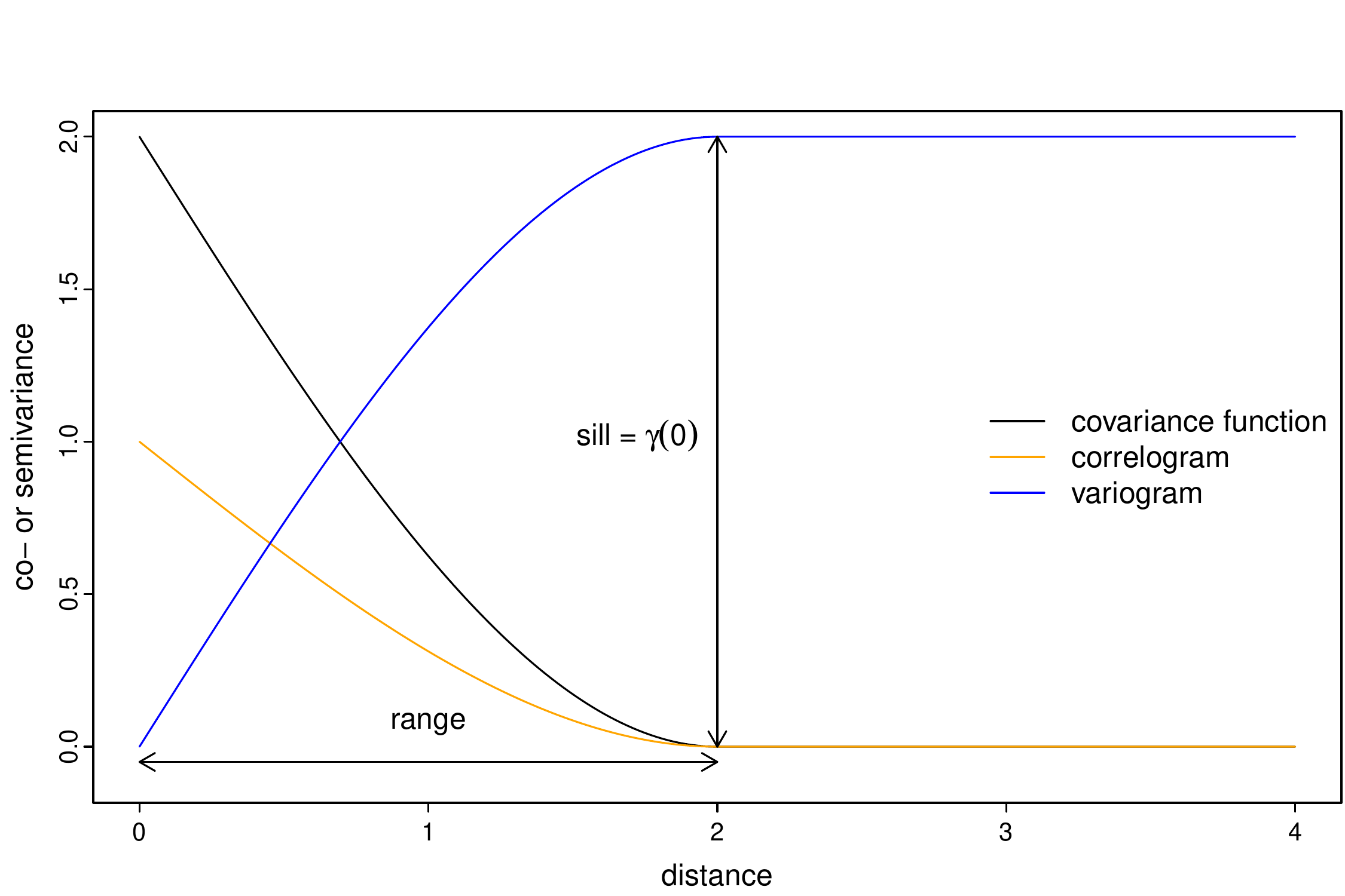
The covariance function describes similarity directly: nearby observations tend to have similar values, so covariance is high at small distances.
The variogram describes dissimilarity: nearby observations tend to have small differences, so the variogram is low at small distances.
So they contain essentially the same information, but in opposite forms: as distance increases, covariance generally decreases while the variogram increases.
The sill corresponds to the variance of the data (\(\gamma(0)\)). The range describes the distance up to which the data points are spatially auto-correlated.
Summary stochastic process
Stochastic process: generalisation of multidimensional random variable
Stationarity assumption required for estimation from single realisation of stochastic process
In practice assumption of weak stationarity:
constant mean
constant variance
covariance and semivariance depends only on lag distance but not on location
Often additional assumption of isotropic auto-correlation