25 Assessment strategies and metrics
Download slides PDF
The PDF contains what was shown during the lecture. This website includes some additional text in light gray.
e-Lecture video
This lecture is available as recording.
25.1 Goal of model assessment
Data analysis often leads to a set of equally plausible candidate models that use different sets of covariates or different approaches to build them.
Summary statistics (like RMSE, R2, kappa) to characterize:
How well does a model fit the data?
Compare models: What is the best model structure, what are relevant covariates? Model selection, variogram functions, tuning parameters.
Evaluate generalization properties: What is the average error to predict for a location without observed data?
Note on model fit
Models with goodness-of-fit metrics often allow model building, but:
Goodness-of-fit not necessarily good criterion for judging quality of predictions.
Predictor selection by
step()does not lead to a unique set of covariates but depends on the search strategy and on criterion (AIC/BIC) used for model section.Likelihood ratio tests cannot be used to compare the goodness-of-fit of models that have different variograms.
Therefore, independent validation or data splitting are required. Machine learning models often directly rely on such techniques as goodness-of-fit criteria do not exist or are not meaningful.
25.2 Model assessment strategies
How to obtain data pairs of observed and predicted?
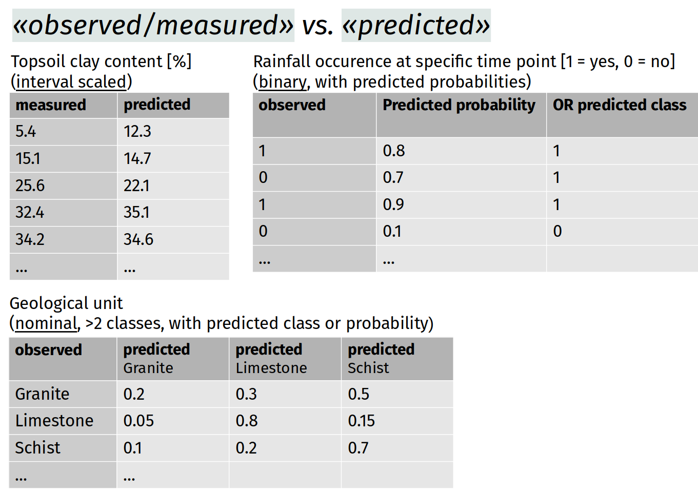
Overview strategies
Completely independent sampling
Splitting of available data
Cross-validation
Non-parametric boostrap
Note: In the classical statistical context an independent data set with which the model performance is evaluated is often called validation set, in machine learning context it is called a test set. The validation set in machine learning is an additional subset of the data, especially often used with to neuronal networks, that serves to find optimal tuning parameters.
Completely independent sampling
→ Desired option
Independent data:
Survey from another institution/database (but, needs to be the same target population and survey method)
New survey:
Independently surveyed from data used for model calibration
Approach to select locations (and depth if 3D): design-based sampling, e.g. stratified random sampling.
Problems
Often no funding for additional survey
Not all studies allow for independent sampling, because it is not meaningful. e.g. landslide occurence is observed whenever it happens.
Not needed, if calibration locations were chosen by a design-based sampling approach, that allows unbiased estimate of model performance metrics, we may use data splitting.
Data splitting
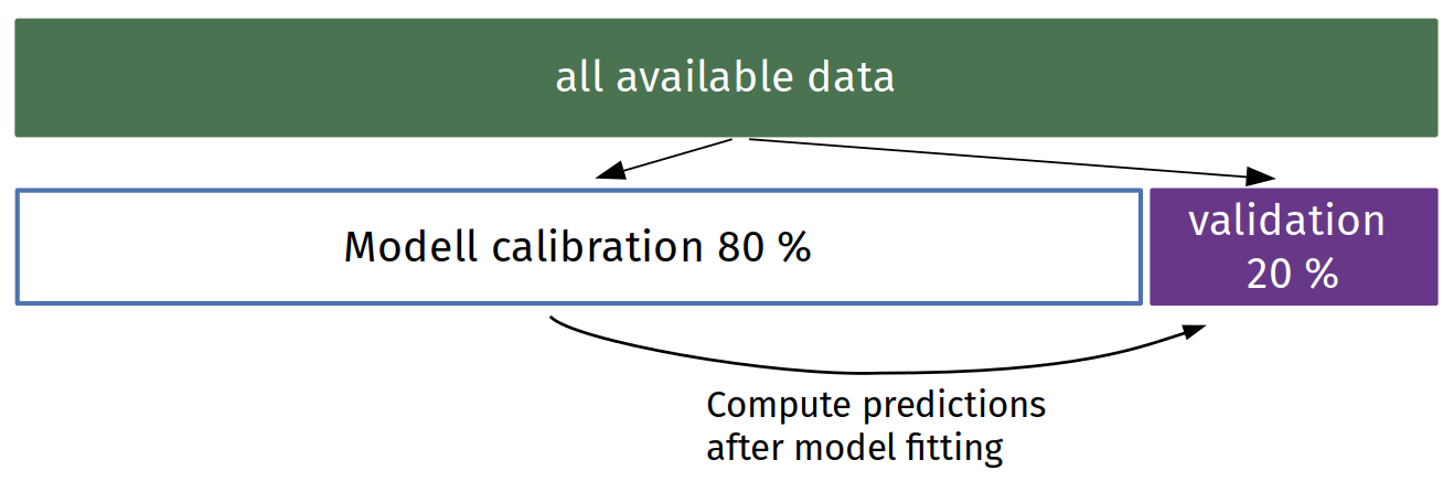
Rule of thumb: 20 % for validation, or a minimal number that allows to compute reliable metrics/means, e.g. 30–50.
How to split:
simple random sample
weighted or stratified random sample, if data does not represent the target population well
Example for weighted splitting
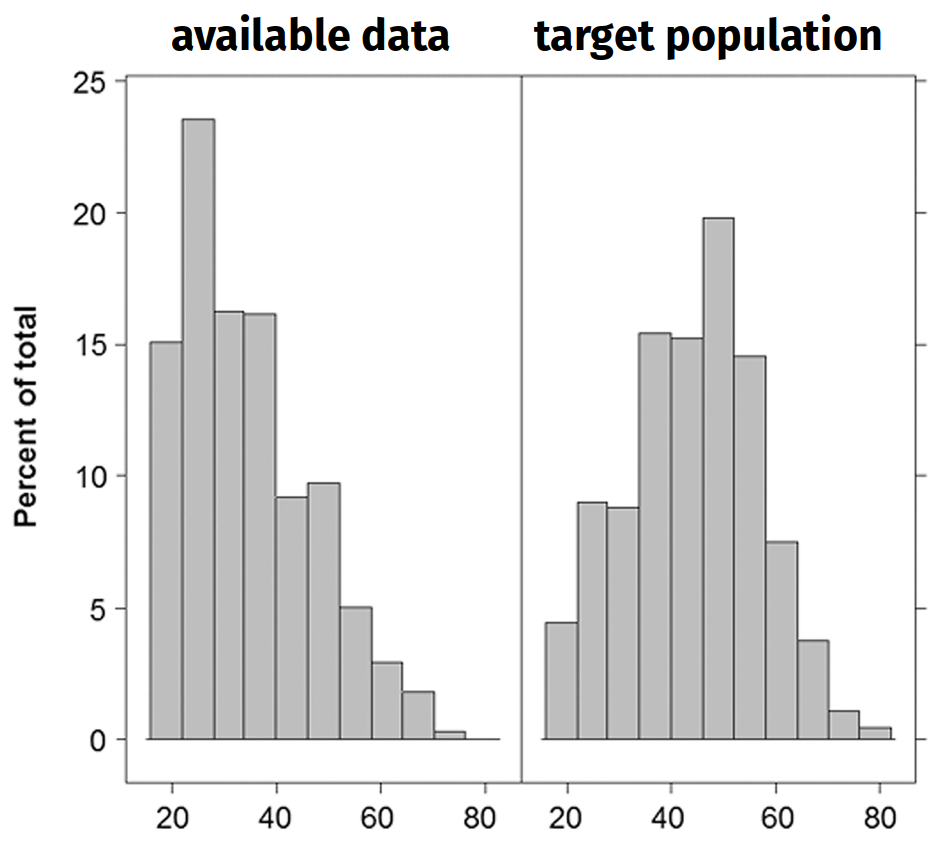
Weighted random sample
Use occurrence probabilities of target population to obtain a validation set with distribution of target population.
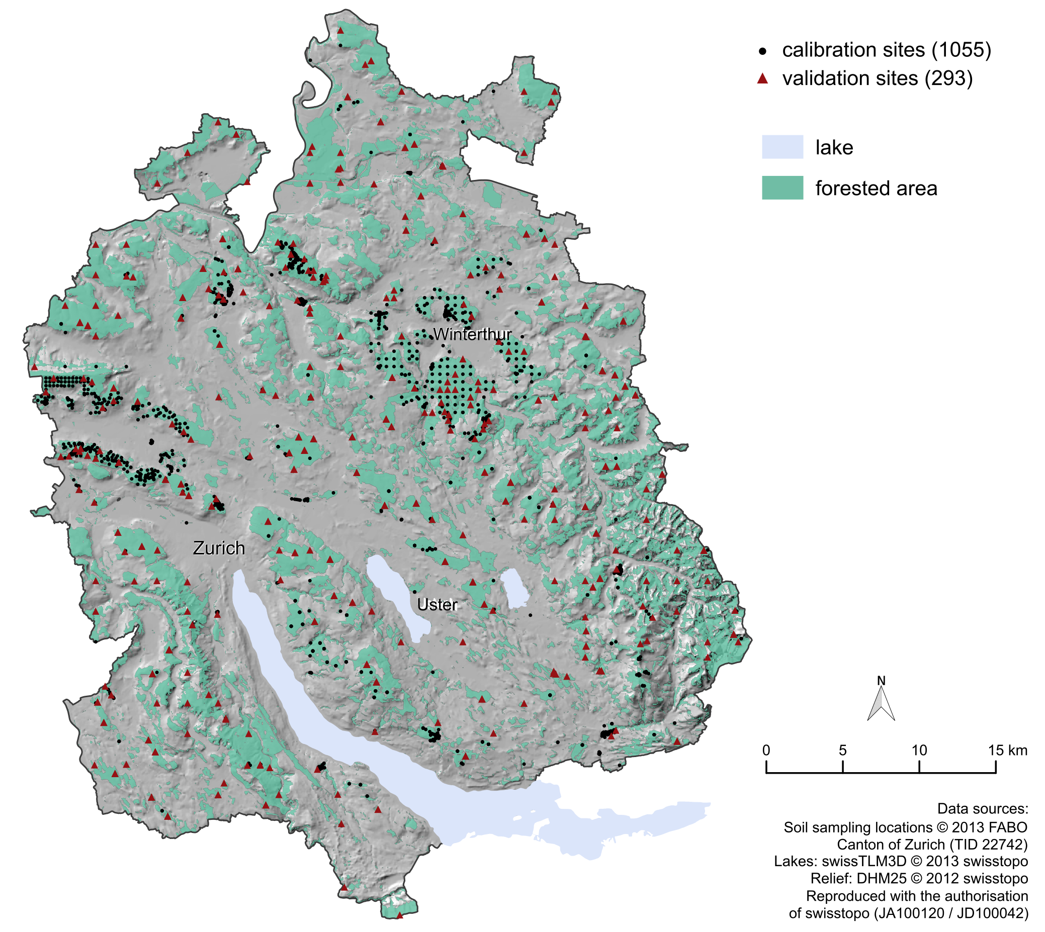
Example for weighted splitting by spatial distribution
Problem: Data from pooled surveys, some strongly spatially clustered. Goal: Prediction for complete forested area of Canton of Zurich
→ Data splitting with weights to obtain homogenouous cover of total study area.
(Weights computed from Thyssen-polygons intersected with the forested area.)
Data splitting – problems
No proper independent data
Sub-optimal variant of new survey
Largely depends how splitting is done
Especially if splitting is done randomly: better to repeat
k-fold cross-validation
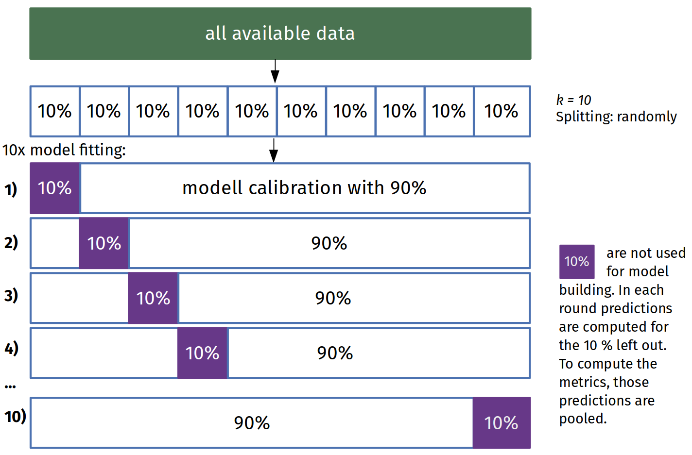
Implementation of k-fold cross-validation
Recommended \(k = 10\) or \(k = 5\) for time-consuming model fits
\(k = n\) is possible (leave-one-out cross-validation), but not recommended due to spatial auto-correlation
Splitting at random or by other criteria possible, e.g. by spatial clusters/blocks.
To allow for comparison of different models cross-validation sets have to be kept fixed.
Repeated cross-validation with repeated splitting of data: Allows to obtain variation of metrics.
Combine with data-splitting: 20 % for validation, 80 % for model selection with cross-validation.
How to do the splitting
Goal of cross-validation strategy
Try to create a similar situation trough data splitting (for e.g. cross-validation) as you have for the prediction of new locations without observations.
If the available data does not allow to reproduce such a situation, results need to be interpreted cautiously!
Spatial cross-validation
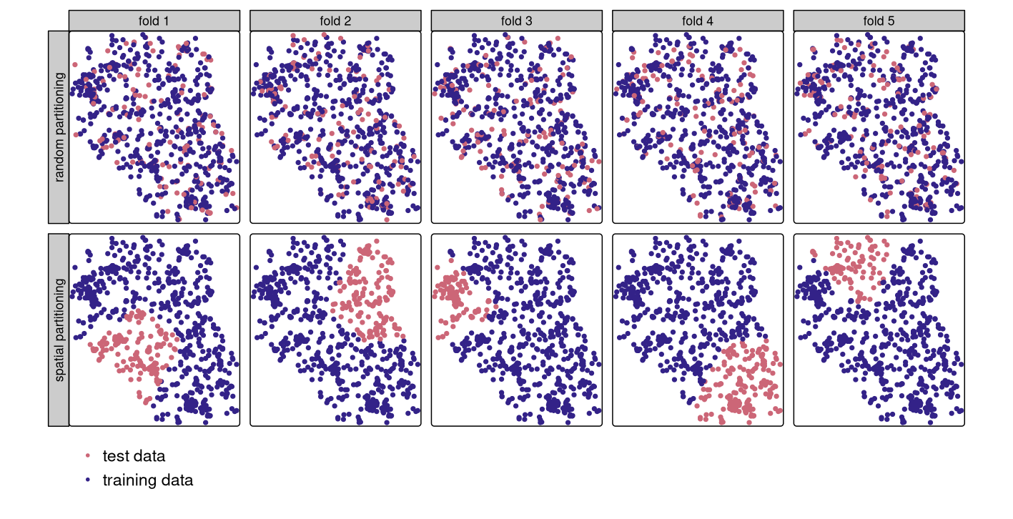
Spatial visualization of selected validation and calibration observations for cross-validation wit random (upper row) and spatial partitioning (lower row).
→ Such a set-up test the extrapolation capacity in an area without any training data. Validation of nearby locations – as many new pixels are between the observed points – is limited.
Spatial or random cross-validation splitting?
Not recommended in general because metrics become too pessimistic – as compared to ideal situation with design-based probability sample.
Splitting by spatial clusters/blocks can be done, e.g. to evaluate spatial extrapolation capacity.
If data is extremely clustered, spatial prediction outside of the observed clusters has to be questioned and should only be done if there is enough domain knowledge to evaluate the outcome (e.g. by asking an expert for meaningfulness)
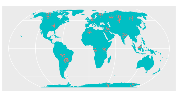
Software for spatial CV:
- Spatial grouping of observation points, e.g. in
cv(.., method = "block")in R packagegeorob. - Further spatial cross-validation in R Packages
mlr3spatiotempcvandCAST.
k-fold cross-validation – Problems
Random splitting: same problem as with data splitting. If available data does not well represent target area/population, validation results might be biased.
If cross-validation has been used for model selection, the final cross-validation results do not yield independent model performance metrics anymore.
Solution: nested cross-validation, inner loop for model selection, outer loop for model evaluation.
Example of wrong use of cross-validation:
Pre-selection of covariates based on correlation coefficient (using all data)
Create \(k\) subsets, fit models by leaving each \(k\) subsets out in turn
Compute predictions for left out subsets, compute error metrics
Non-parametric bootstrap
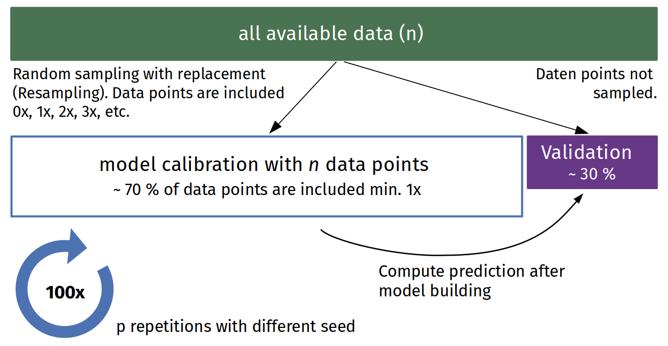
Problems:
Random splitting of biased data: same problem as for data-splitting or cross-validation.
Larger number of models needed.
Potential: simulate standard errors or prediction intervals for models that do not provide these.
Bootstrap corresponds to out-of-bag predictions in random forest.
25.3 Model assessment metrics and displays
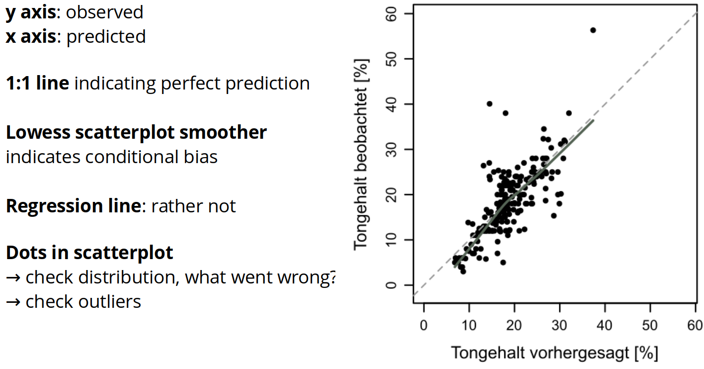
Interval scaled response – validation scatterplot
Interval scaled response – metrics
To summarized the validation scatterplot, it is recommended to report at least 3 metrics:
a bias metric, indicating marginal bias
an overall precision statistic, reporting the standard deviation of the errors in the original unit of the response (bias and random variation)
a standardized error statistic, comparable across datasets.
Often reported are mean error (ME) or bias, root mean squared error (RMSE) and R2.
Interval scaled response – metrics Bias and RMSE
With \(y_{i}\) being the observed value at location \(i\) and \(\hat{Y}(\mathbf{x}_{i})\) the predicted map at location \(i\).
Bias (positive: over-prediction, negative: under-prediction):
\[ \mathrm{BIAS} = \frac{1}{n}\sum_{i=1}^n \left( \hat{f}(\mathbf{x}_{i})-y_{i}\right) \]
Root mean square error:
\[ \mathrm{RMSE} = \sqrt{\frac{1}{n}\sum_{i=1}^n \left( \hat{f}(\mathbf{x}_{i})-y_{i}\right)^2} \]
Interval scaled response – metrics R2
R2 (also model efficiency coefficient or mean squared error skill score) with \(\overline{y}\) being the mean of the observed data
\[ \mathrm{R^2} = 1 - \frac{\sum_{i=1}^n \left( y_{i}-\hat{f}(\mathbf{x}_{i})\right)^2}{\sum_{i=1}^n \left( y_i - \overline{y} \right)^2} \]
1: perfect prediction.
0: mean squared error is the same as variance of observed data, i.e. a map showing the mean of the data would have the same average prediction performance.
<0: mean squared error is larger than variance of observed data.
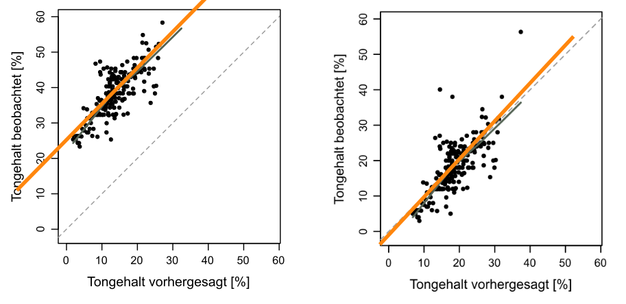
Interval scaled response – R2 vs. r2
\(R^2 \ne r^2\).
R2 does not correspond to Pearson correlation coefficient in presence of bias.
Binary responses – confusion matrix
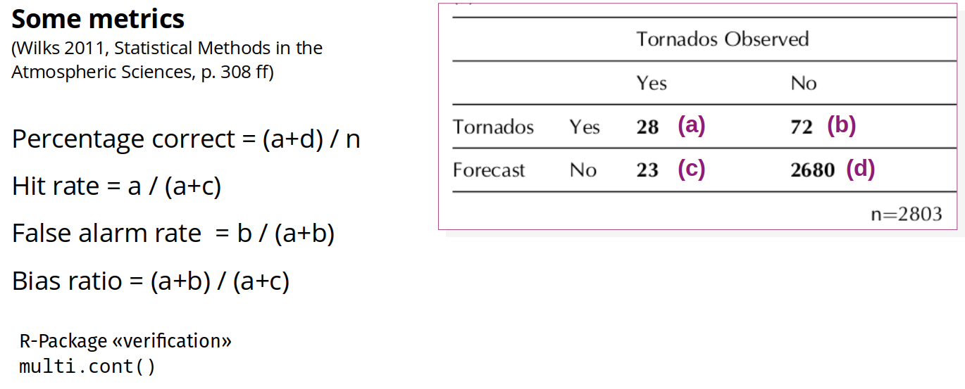
Binary responses – confusion matrix
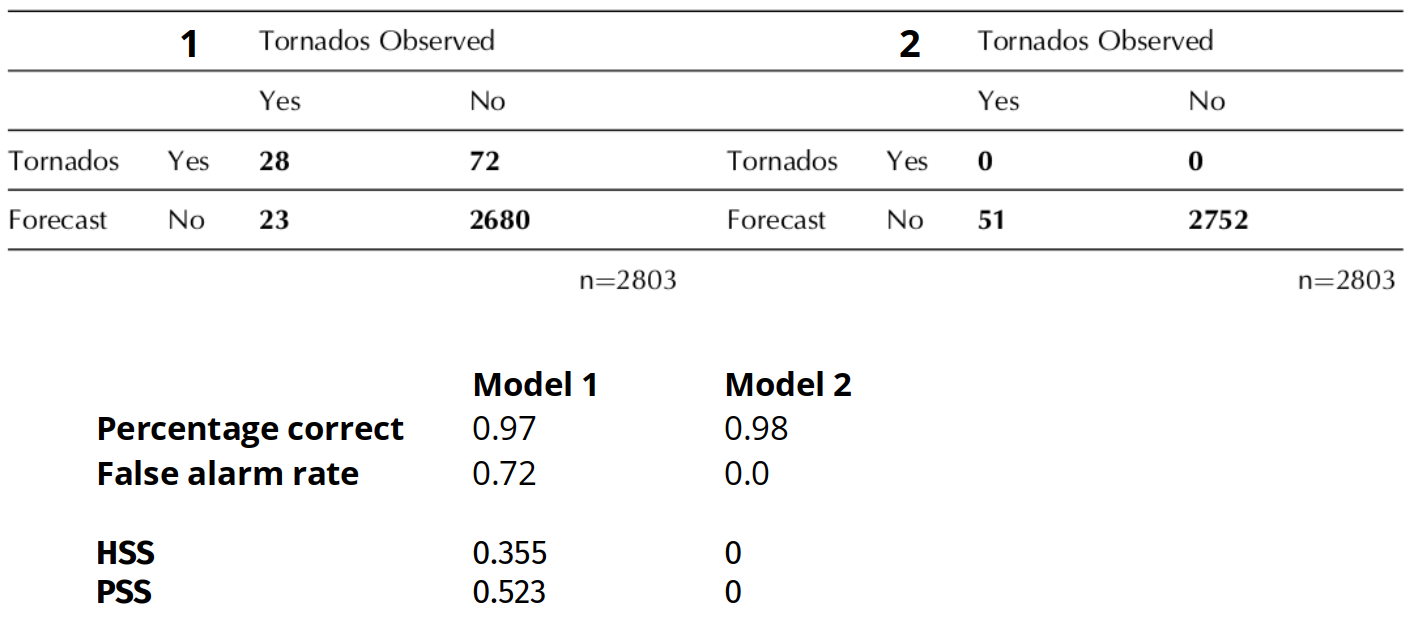
Hedging / “gaming” the score: Uninformative predictions yield good scores. Alternative: Skill scores for confusion matrices, e.g.:
HSS: Heidke skill score (also kappa)
PSS: Pierce skill score
Binary responses – Pierce skill score
Pierce skill score (simplified notation):
\[ PSS = \frac{ad - bc}{(a+c)(b+d)} \]
Reference: random predictions that are constrained to be unbiased.
Score range \([-1,1]\):
1: perfect prediction
0: prediction equal to random class assignment
-1: prediction always opposite of observed class
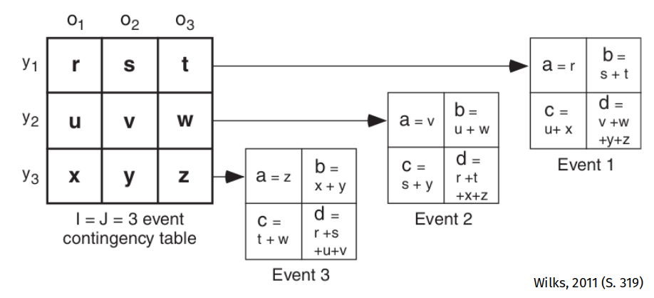
Multinomial responses – extension of binary case
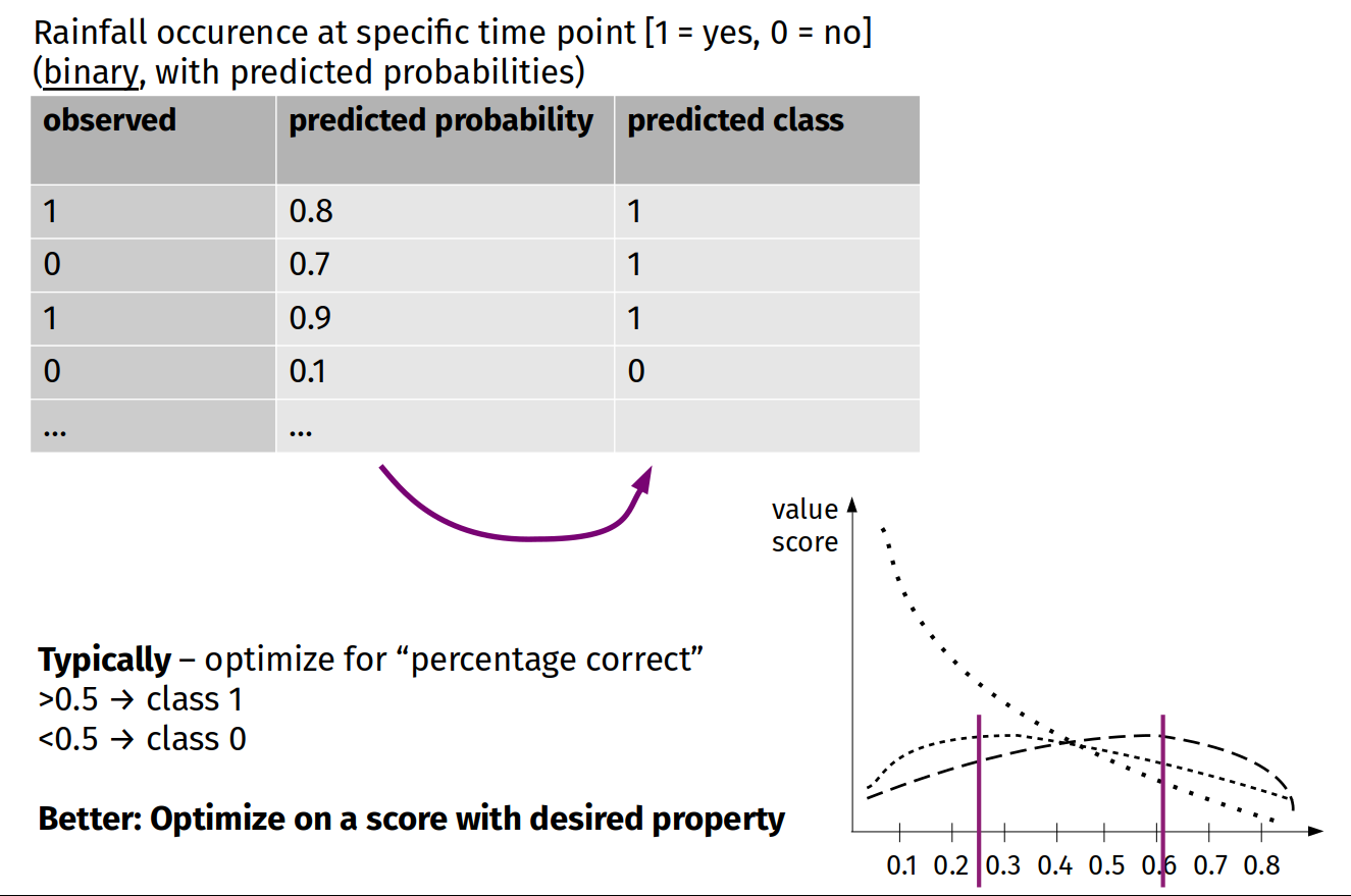
Use score to optimally discretize predictions
25.4 Summary
Strategies to form pairs of predicted and observed
- New independent sampling
- Splitting of available data once
- Splitting of available data multiple times
- Cross-validation
- Bootstrap
→ Spatial location can be considered in splitting. But, most often not needed.
Validation plots and metrics
- Continious intervalscaled response: scatterplot, bias, RMSE, R^2
- Categorical response: confusion matrix, bias ratio, percentage correct, skill scores like PSS
→ Other metrics might be common in your domain (like F1 score). Then also report these.