plot(r.georob.ml, lag.dist.def=20, max.lag=200)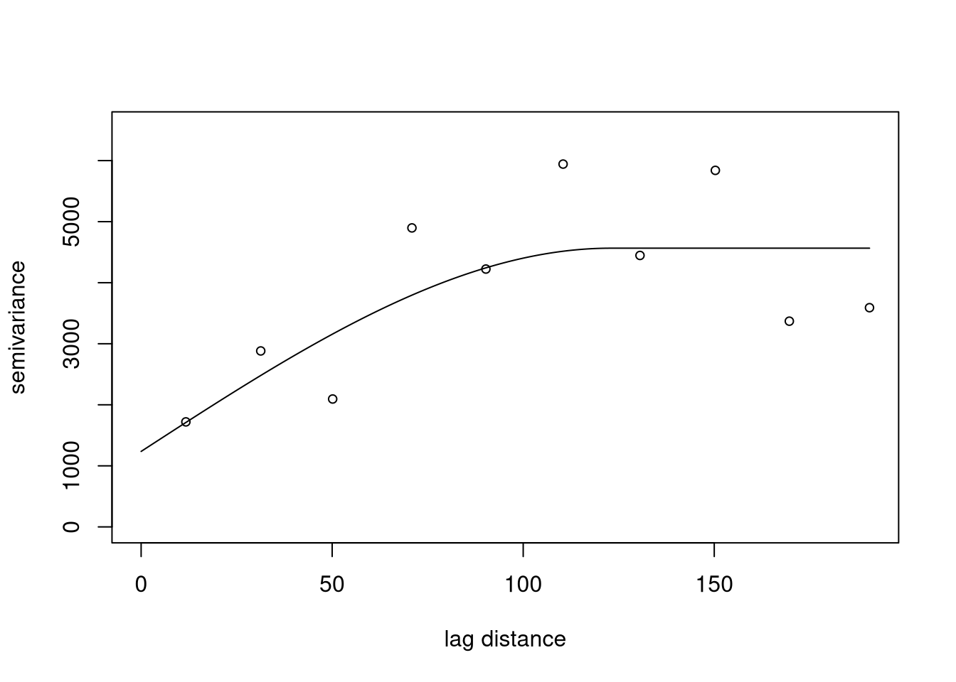
This chapter contains a more technical version of chapter 8. The same topics are covered.
Download slides PDF
The PDF contains what was shown during the lecture. Some of these websites include additional text in light gray.
Model for data: \(Y_{i} = S(\mathbf{x}_{i}) + Z_{i} = \mu(\mathbf{x}_{i}) + E(\mathbf{x}_{i}) + Z_{i}\)
with \(Y_{i}\): \(i^{\text{th}}\) datum; \(S(\mathbf{x}_{i})\): “signal” (true quantity) at location \(\mathbf{x}_{i}\); \(\mu(\mathbf{x}_{i})\): trend
\(\{E(\mathbf{x}_{i})\}\): a zero-mean Gaussian process, parametrized by covariance function \(\gamma(\mathbf{h}; \mathbf{\theta})\) or variogram \(V(\mathbf{h}; \mathbf{\theta})\)
\(Z_{i}\): iid Gaussian measurement error with variance \(\tau^2\)
Trend \(\mu(\mathbf{x}_{i})\) modeled by linear regression model with spatial covariates \(d_{k}(\mathbf{x}_{i})\)
\[ \mu(\mathbf{x}_{i}) = \sum_{k} d_{k}(\mathbf{x}_{i}) \beta_{k} = \mathbf{d}(\mathbf{x}_{i})^{T} \mathbf{\beta} \]
Unknown elements of the model:
Structure and parameters \(\mathbf{\beta}\) of the trend model
Covariance (or variogram) parameters \(\mathbf{\theta}\)
Nugget variance \(\tau^2\)
Ordinary least squares (OLS) trend estimation
Gaussian model in vector notation: \(\mathbf{Y} = \mathbf{X} \mathbf{\beta} + \mathbf{E} + \mathbf{Z}\)
Estimation of trend parameters \(\mathbf{\beta}\) by ordinary least squares:
\[ \hat{\mathbf{\beta}}_{\text{OLS}} = (\mathbf{X}^\top \mathbf{X})^{-1} \mathbf{X}^\top \mathbf{Y} \]
For spatially uncorrelated data (\(\mathbf{E} = \mathbf{0}\); \(\text{Cov}(\mathbf{Y}, \mathbf{Y}^\top) = \tau^2 \mathbf{I}\)):
\[ \hat{\mathbf{\beta}}_{\text{OLS}} \sim \mathcal{N}\left(\mathbf{\beta}, \tau^2 (\mathbf{X}^\top \mathbf{X})^{-1} \right) \]
\(\tau^2\mathbf{I}\) represents independent error: every observation has error variance \(\tau^2\), but the errors are uncorrelated with each other (\(\mathbf{I}\): identity matrix with \(\tau^2\) on the diagonal and zero elsewhere).
For spatially auto-correlated data \(\text{Cov}(\mathbf{Y}, \mathbf{Y}^\top) = \text{Cov}(\mathbf{Z}, \mathbf{Z}^\top) + \text{Cov}(\mathbf{E}, \mathbf{E}^\top) = \mathbf{\Gamma}_{\theta} = \tau^2 \mathbf{I} + \mathbf{\Sigma}_{\theta}\)
\[ \hat{\mathbf{\beta}}_{\text{OLS}} \sim \mathcal{N}\left(\mathbf{\beta}, \tau^2(\mathbf{X}^\top \mathbf{X})^{-1} + (\mathbf{X}^\top \mathbf{X})^{-1} \mathbf{X}^\top \mathbf{\Sigma}_{\theta} \mathbf{X} (\mathbf{X}^\top \mathbf{X})^{-1} \right) \]
Conclusion: Ignoring auto-correlation: \(\hat{\mathbf{\beta}}_{\text{OLS}}\) unbiased, but the standard errors are too small. Tests based on OLS fit are biased!
OLS assumes independent errors. The covariance matrix \(\tau^2I\) expresses equal error variance \(\tau^2\) and zero covariance between observations. For spatial data, observations may additionally share spatially correlated variation, represented by the covariance matrix \(\Sigma_\theta\). The OLS coefficient estimates can still be unbiased if the spatial process has zero mean and is unrelated to the covariates, but the usual OLS variance formula ignores \(\Sigma_\theta\). Consequently, standard errors and statistical tests can be incorrect.
Generalized least squares (GLS) trend estimation
Generalized least squares estimates:
\[ \hat{\mathbf{\beta}}_{\text{GLS}} = (\mathbf{X}^\top \mathbf{\Gamma}_{\theta}^{-1} \mathbf{X})^{-1} \mathbf{X}^\top \mathbf{\Gamma}_{\theta}^{-1} \mathbf{Y} \]
GLS = OLS with “orthogonalized” response and design matrix.
Sampling distribution:
\[ \hat{\mathbf{\beta}}_{\text{GLS}} \sim \mathcal{N}\left(\mathbf{\beta}, (\mathbf{X}^\top \mathbf{\Gamma}_{\theta}^{-1} \mathbf{X})^{-1} \right) \]
For spatially uncorrelated data (\(\mathbf{\Gamma}_{\theta} = \tau^2 \mathbf{I}\)):
\[ \hat{\mathbf{\beta}}_{\text{GLS}} = \hat{\mathbf{\beta}}_{\text{OLS}} \]
\(\hat{\mathbf{\beta}}_{\text{GLS}}\) has the smallest standard errors among all linear estimators (Gauss-Markov theorem), hence it’s the BLUE (Best Linear Unbiased Estimator).
\(\hat{\mathbf{\beta}}_{\text{GLS}}\) is the maximum likelihood estimate for Gaussian \(\mathbf{Y}\).
Generalised least squares (GLS) is the method of choice for estimating coefficients of the trend model.
Sample variogram (also experimental variogram) consists of semivariances at a finite set of discrete lags \(h\).
Underlying function is continuous for all \(h\).
Variogram modelling:
Compute sample variogram
Fit smooth function that describes principal features of semivariance sequence
Extract residuals \(\mathbf{R} = \mathbf{Y} - \mathbf{X} \hat{\mathbf{\beta}}\) of the fitted linear model (or use data \(\mathbf{Y}\) if the model has constant \(\mu(\mathbf{x})\)).
Choose bin width \(dh\) (and width of angular classes \(d\phi\)) to define the \((k,l)^{\text{th}}\) lag class, \(\mathbf{h}_{kl}\), characterized by:
Distance: \((h_k - dh, h_k + dh]\)
Angular class: \(\phi_l - d\phi, \phi_l + d\phi\)
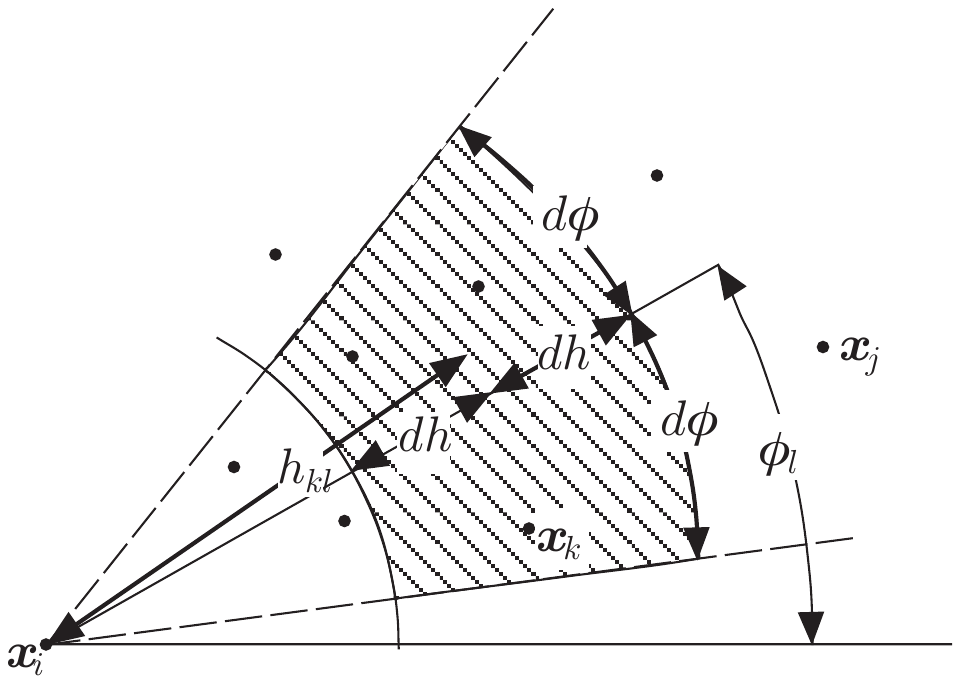
Form all \(N_{kl}\) pairs \((i,j)\) with \(\mathbf{x}_{i} - \mathbf{x}_{j} \approx \mathbf{h}_{kl}\).
Compute for each lag class \(\mathbf{h}_{kl}\) the semivariance: \[ \hat{V}(\mathbf{h}_{kl}) = \frac{1}{2 N_{kl}} \sum_{(i,j) \in \mathbf{h}_{kl}} \left[R(\mathbf{x}_{i}) - R(\mathbf{x}_{j})\right]^2 \]
Sample variogram: Plot of \(\hat{V}(\mathbf{h}_{kl})\) vs. \(\mathbf{h}_{kl}\).
Rules of thumb:
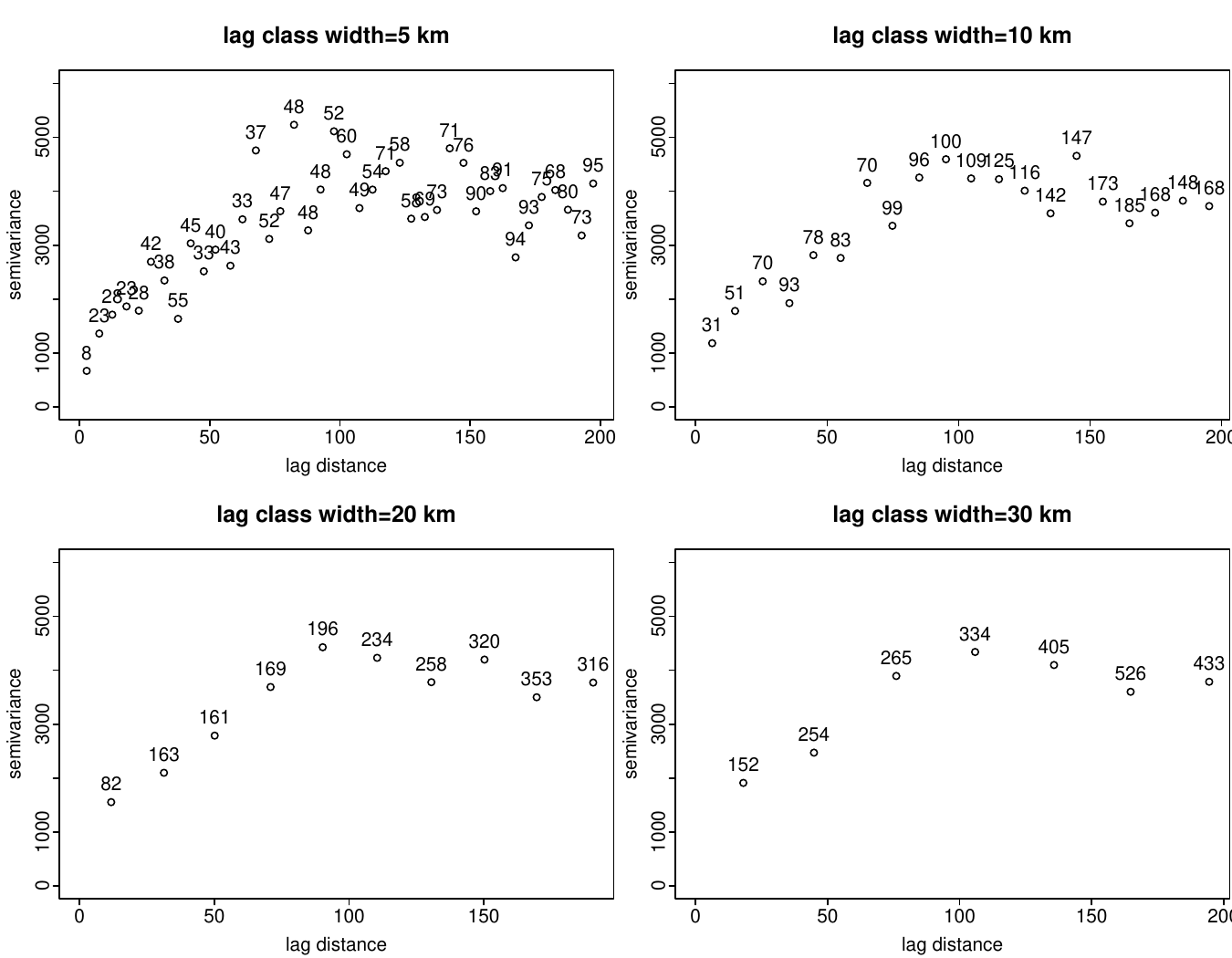
Ensure enough data pairs per lag class. Choose \(dh\) (and \(d\phi\)) such that \(N_{kl} > 30-50\).
Only compute the variogram for half the size of the study area.
Largest \(\mathbf{h}_{kl} \leq 0.5 \max(\mathbf{x}_{i} - \mathbf{x}_{j})\).
Semivariance is required for arbitrary lag distances when computing predictions.
Smoothing the sample variogram by fitting a parametric variogram function \(V(\mathbf{h}, \mathbf{\theta})\).
Choose a variogram function that approximates the shape of the sample variogram well, particularly close to the origin.
Fit parameters \(\mathbf{\theta}\) by (weighted) least squares: \[ \hat{\mathbf{\theta}} = \underset{\mathbf{\theta}}{\text{argmin}} \sum_{kl} w(\mathbf{h}_{kl}) \left( V(\mathbf{h}_{kl}) - \hat{V}(\mathbf{h}_{kl}, \mathbf{\theta}) \right)^2 \]
Options for weighing:
Equal weights: \(w(\mathbf{h}_{kl}) = 1\)
By number of pairs: \(w(\mathbf{h}_{kl}) = N_{kl}\)
Cressie’s weights: \(w(\mathbf{h}_{kl}) = \frac{N_{kl}}{V(\mathbf{h}_{kl}, \mathbf{\theta})^2}\)
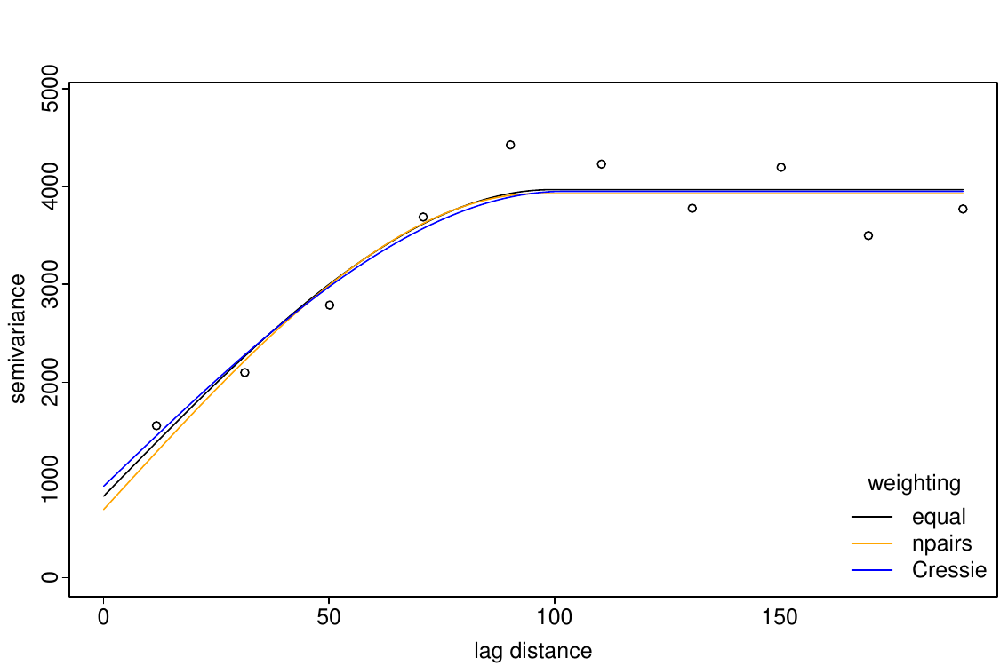
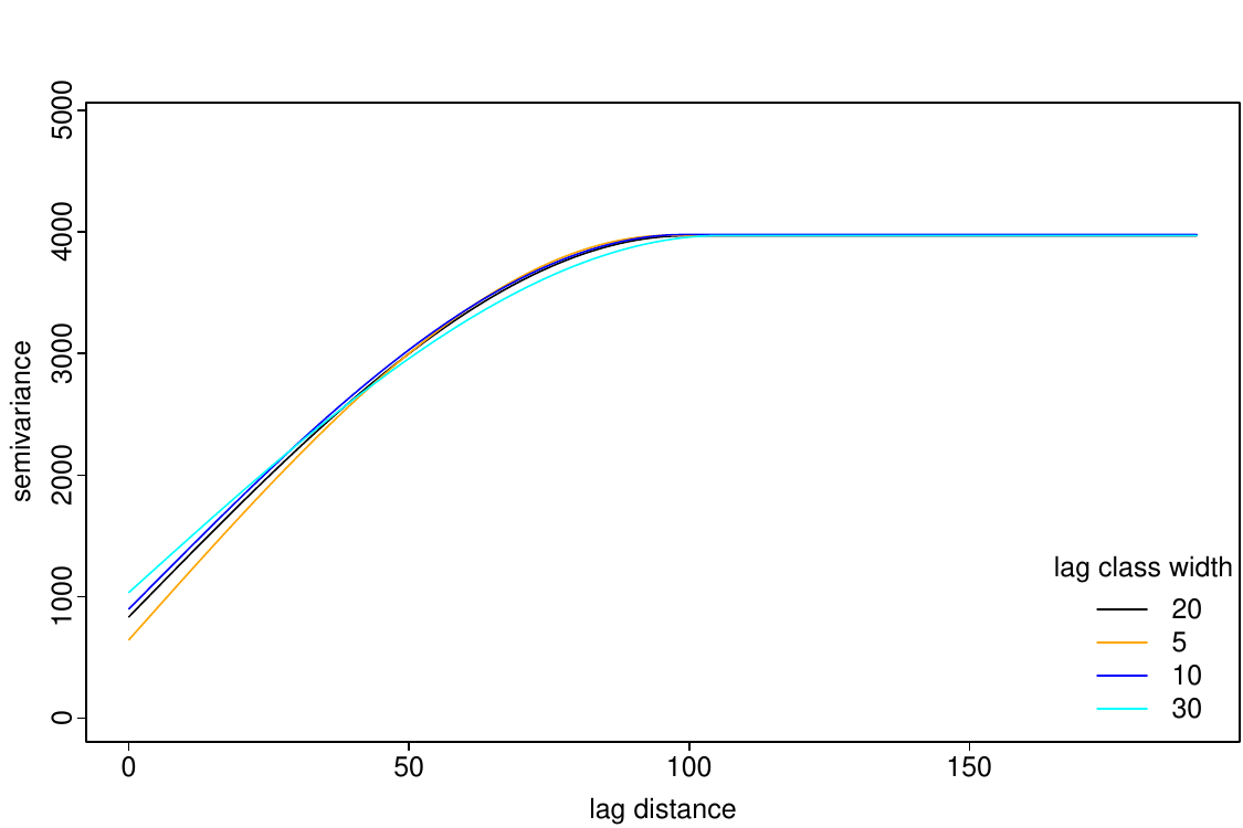
Subjective choice of lag class width and weighting method for model fitting.
Estimates of semivariance for different lag classes are mutually correlated; the choice of variogram function based on the sample variogram is problematic.
The sample variogram is susceptible to outliers, hence robust estimators are preferred.
Fitting a model function to the sample variogram requires further subjective choices.
An ad-hoc approach provides biased estimates of the variogram of the underlying stochastic process if the trend is modeled.
Therefore, the estimate of the variogram based on the sample variogram of OLS residuals is biased.
Thus, estimate trend and variogram parameters simultaneously using maximum likelihood.
Principle of maximum likelihood estimation: find parameters that maximize joint probability for observed data
Properties of maximum likelihood estimates: asymptotically unbiased and fully efficient; asymptotically normally distributed
profile likelihood useful for exploring shape of likelihood surface and for computing confidence intervals based on likelihood ratio test
Consider a Gaussian stochastic process \(\{Y(\mathbf{x})\}\) with a linear trend function.
Any arbitrary set of random variables \(\mathbf{Y} = (Y(\mathbf{x}_{1}), \ldots, Y(\mathbf{x}_{n}))\) has a multivariate Gaussian distribution with expectation: \[
\mathbb{E}[\mathbf{Y}] = \mathbf{X} \mathbf{\beta}
\]
and covariance matrix: \[
\text{Cov}(\mathbf{Y}, \mathbf{Y}^\mathrm{T}) = \mathbf{\Gamma}_{\mathbf{\theta}}
\]
The joint probability density for \(\mathbf{Y}\) is given by:
\[ f(\mathbf{y};\mathbf{\beta},\mathbf{\theta}) = (2\pi)^{-\frac{n}{2}} |\mathbf{\Gamma}_{\mathbf{\theta}}|^{-\frac{1}{2}} \exp\left(-\frac{1}{2} \{\mathbf{y} - \mathbf{X}\mathbf{\beta}\}^\mathrm{T} \mathbf{\Gamma}_{\mathbf{\theta}}^{-1} \{\mathbf{y} - \mathbf{X}\mathbf{\beta}\}\right) \]
Direct ad-hoc variogram fitting: Pairwise information is first aggregated into distance classes (lag), so the result depends on choices such as lag width and maximum lag distance.
Maximum likelihood: The covariance model is fitted directly to the observations. The actual pairwise distances enter the covariance matrix \(\mathbf{\Gamma}_{\mathbf{\theta}}\) and are direclty considered in the model, so no arbitrary lag-distance classes are required.
Note: MLE is not completely assumption-free. You still have to choose the covariance model (e.g. exponential, Matérn) and the structure of the trend function (e.g. linear model).
Maximum likelihood estimation (cont.)
Unknown model parameters:
Regression coefficients \(\mathbf{\beta}\)
Covariance (or variogram) parameters \(\mathbf{\theta}\)
The log-likelihood function (up to a constant) is given by: \[ L(\mathbf{\beta}, \mathbf{\theta};\mathbf{y}) = -\frac{1}{2} \log(|\mathbf{\Gamma}_{\mathbf{\theta}}|) -\frac{1}{2} \{\mathbf{y} - \mathbf{X}\mathbf{\beta}\}^\mathrm{T} \mathbf{\Gamma}_{\mathbf{\theta}}^{-1} \{\mathbf{y} - \mathbf{X}\mathbf{\beta}\} \]
For known variogram parameters \(\mathbf{\theta}\) maximum likelihood estimate for \(\mathbf{\beta}\) equals GLS estimator: \[ \hat{\mathbf{\beta}}_{\mathrm{GLS}} = (\mathbf{X}^\mathrm{T} \mathbf{\Gamma}_{\mathbf{\theta}}^{-1} \mathbf{X})^{-1} \mathbf{X}^\mathrm{T} \mathbf{\Gamma}_{\mathbf{\theta}}^{-1} \mathbf{Y} \]
Plugging \(\hat{\mathbf{\beta}}_{\mathrm{GLS}}\) into \(L(\mathbf{\beta}, \mathbf{\theta};\mathbf{y})\) gives the profile likelihood function for \(\mathbf{\theta}\).
No closed form expression for maximum likelihood estimate
Maximize \(L\) numerically by a non-linear optimization method to find \(\hat{\theta}\)
Numerical optimization requires initial values of \(\theta\)
Make sure numerical optimization converged!
Numerical estimation of the spatial covariance parameters
Starting from initial values for the covariance parameters \(\theta\), a covariance matrix \(\Gamma_\theta\) is constructed. Given this covariance structure, the trend parameters \(\hat{\mathbf{\beta}}_{\mathrm{GLS}}\) are estimated by generalized least squares (GLS). The resulting residuals are then used to update the covariance parameters \(\hat{\theta}\). This procedure is repeated until the parameter estimates converge.
Initial \(\theta\) parameters to start the procedure can be derived by e.g. visually inspecting the variogram of OLS residuals.
R function georob() does the iterative fitting for us. With param the starting values are given. The output indicates if the approximation converged. If not, starting values need to be adapted.
library(gstat); library(georob)
data("wolfcamp"); d.w <- wolfcamp
coordinates(d.w) <- c("x", "y")
r.georob.ml <- georob(pressure~x+y, d.w,
  locations=~x+y, variogram.model="RMspheric",
  param=c(variance=3000, nugget=1000, scale=100),
  tuning.psi=1000, control=control.georob(ml.method="ML"))
summary(r.georob.ml)
Call:georob(formula = pressure ~ x + y, data = d.w, locations = ~x +
    y, variogram.model = "RMspheric", param = c(variance = 3000,
    nugget = 1000, scale = 100), tuning.psi = 1000, control = control.georob(ml.method = "ML"))

Tuning constant:  1000

Convergence in 12 function and 7 Jacobian/gradient evaluations

Estimating equations (gradient)

                                 eta         scale
  Gradient           : -8.880367e-05  7.654524e-04

Maximized log-likelihood: -458.3671

Predicted latent variable (B):
   Min     1Q Median     3Q    Max
-89.37 -54.98 -16.64  24.43 111.41

Residuals (epsilon):
    Min      1Q  Median      3Q     Max
-62.789 -19.775   6.311  18.032  62.776

Standardized residuals:
    Min      1Q  Median      3Q     Max
-2.3778 -0.7413  0.2249  0.6534  3.2793


Gaussian ML estimates

Variogram:  RMspheric
               Estimate   Lower  Upper
variance        3328.90 1453.95 7621.7
snugget(fixed)     0.00      NA     NA
nugget          1236.27  616.01 2481.1
scale            122.95   95.13  158.9


Fixed effects coefficients:
            Estimate Std. Error t value Pr(>|t|)
(Intercept) 620.3550    17.0641  36.354  < 2e-16 ***
x            -1.3256     0.1360  -9.750 2.33e-15 ***
y            -1.2061     0.1793  -6.727 2.16e-09 ***
---
Signif. codes:  0 '***' 0.001 '**' 0.01 '*' 0.05 '.' 0.1 ' ' 1

Residual standard error (sqrt(nugget)): 35.16

Robustness weights:
All 85 weights are ~= 1.plot(r.georob.ml, lag.dist.def=20, max.lag=200)
Equivalent number of independent observations of a sample of spatial data often much smaller than nominal sample size ⇒ bias of maximum likelihood estimates of variance parameters important
The bias of MLEs of variogram parameters \(\mathbf{\theta}\) can be reduced by restricted maximum likelihood estimation (REML).
Principle of REML:
The matrix \(\mathbf{A}\) must satisfy: \(\mathbf{A} \mathbf{X} = \mathbf{0}\)
\(\mathbf{A}\) is non-unique with many possibilities
GLS accounts for spatial redundancy when estimating the trend parameters \(\beta\), but MLE can still underestimate variance and covariance parameters \(\theta\) because the effective number of independent observations is smaller than the nominal sample size.
REML accounts for the loss of degrees of freedom from estimating the trend, reducing the small-sample bias of ML estimates of variance parameters.
This georob() function call is basically the work-horse of our geostatistical model fitting. REML is the default and does not need to be specified separately.
r.georob.reml <- georob(pressure~x+y, d.w,
  locations=~x+y, variogram.model="RMspheric",
  param=c(variance=3000, nugget=1000, scale=100),
  tuning.psi=1000)
summary(r.georob.reml)
Call:georob(formula = pressure ~ x + y, data = d.w, locations = ~x +
    y, variogram.model = "RMspheric", param = c(variance = 3000,
    nugget = 1000, scale = 100), tuning.psi = 1000)

Tuning constant:  1000

Convergence in 6 function and 5 Jacobian/gradient evaluations

Estimating equations (gradient)

                                 eta         scale
  Gradient           : -2.248651e-04 -1.070402e-01

Maximized restricted log-likelihood: -456.3802

Predicted latent variable (B):
   Min     1Q Median     3Q    Max
-94.58 -60.99 -17.59  23.10 115.72

Residuals (epsilon):
    Min      1Q  Median      3Q     Max
-59.148 -18.009   6.251  15.982  54.620

Standardized residuals:
    Min      1Q  Median      3Q     Max
-2.4030 -0.7131  0.2282  0.6937  3.1932


Gaussian REML estimates

Variogram:  RMspheric
               Estimate   Lower   Upper
variance        4358.84 1810.40 10494.6
snugget(fixed)     0.00      NA      NA
nugget          1151.28  540.41  2452.7
scale            138.91   82.62   233.6


Fixed effects coefficients:
            Estimate Std. Error t value Pr(>|t|)
(Intercept) 624.3287    20.7961  30.021  < 2e-16 ***
x            -1.3291     0.1611  -8.248 2.25e-12 ***
y            -1.1804     0.2115  -5.581 3.00e-07 ***
---
Signif. codes:  0 '***' 0.001 '**' 0.01 '*' 0.05 '.' 0.1 ' ' 1

Residual standard error (sqrt(nugget)): 33.93

Robustness weights:
 All 85 weights are ~= 1.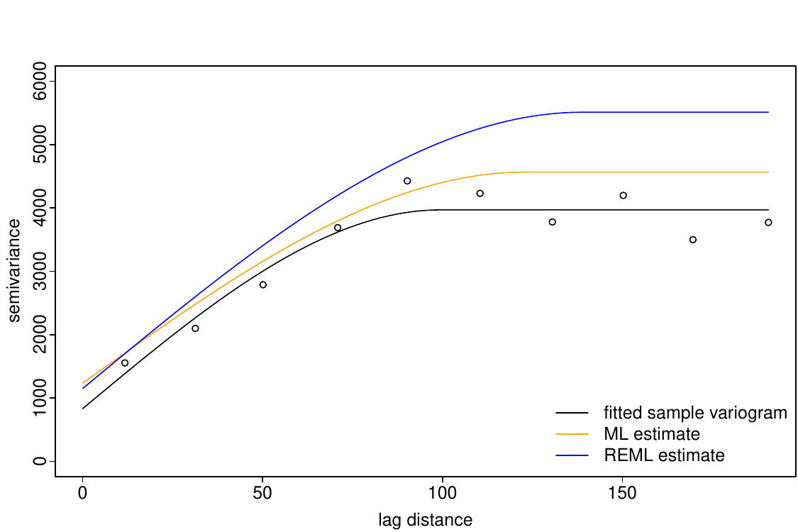
Different estimation methods can give different sill estimates. Variogram fitting depends on the chosen lag classes and weighting (binning often reduces variance), whereas ML and REML use the full spatial covariance structure. ML tends to underestimate variance parameters in finite samples. REML corrects for the loss of degrees of freedom due to estimating the trend, often resulting in a larger sill.