The PDF contains what was shown during the lecture. Some of these websites include additional text in light gray.
4.1 Geostatistical model notation
Objectives of geostatistical analyis
Computing spatial predictions of response variable for
a location without measurement, i.e. a creating spatially continuous surface
finite support targets (spatial means)
2. Quantifying uncertainty of these predictions
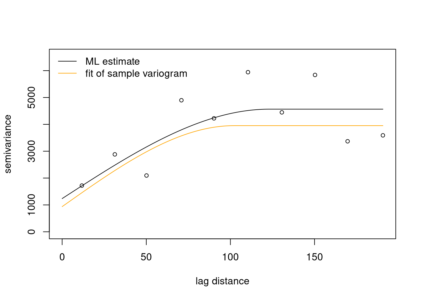
3. Estimation of parameters of (regression) models fitted to geostatistical data
Geostatistical data sets
Set of observations \((y_i, \mathbf{x}_i)\) where \(y_i\) is a datum of a response variable and \(\mathbf{x}_i\) is a spatial location in a study domain \(D\)
Optional: spatial covariates, say \(d_k(\mathbf{x}_i)\), used to “explain” the spatial pattern of the response variable
Geostatistical data often show (gradual) large-scale spatial variation and small-scale local fluctuations
trend: commonly modelled as low-order polynomial function of spatial coordinates (⇒ trend surface) or as function of external spatial covariates (⇒ external trend)
local fluctuations usually spatially structured (values at pairs of nearby locations “more similar” than for pairs farther apart) ⇒ spatial auto-correlation
Spatial data is sometimes distorted by independent measurement errors
Terminology and model notation
Model for data: \(Y_{i} = S(\mathbf{x}_{i}) + Z_{i}\)
where
\(Y_{i}\) : \(i^\mathrm{th}\) datum
\(S(\mathbf{x}_{i})\) : “signal” (= true quantity) at location \(\mathbf{x}_{i}\)
\(Z_{i}\) : iid. random measurement error
Decomposition of signal into trend \(\mu(\mathbf{x}_{i})\) and stochastic fluctuation:
where commonly a linear model is used for \(\mu(\mathbf{x}_{i})\)
\[
\mu(\mathbf{x}_{i}) = \sum_{k} d_{k}(\mathbf{x}_{i}) \beta_{k} =
\mathbf{d}(\mathbf{x}_{i})^\mathrm{T} \mathbf{\beta}
\] with \(d_{k}(\mathbf{x}_{i})\) denoting (spatial) covariates and \(\{E(\mathbf{x}_{i})\}\) a zero mean stochastic process (random field).
In summary
Geostatistical data (\(y_i\) , \(\mathbf{x}_i\), \(d_k(\mathbf{x}_i)\)):
response \(y_i\)
location \(\mathbf{x}_i\)
covariates \(d_k(\mathbf{x}_i)\)
often approximately infinitesimal support
‘Approximately infinitesimal support’ means that a measurement is assumed to represent the value at a specific location, rather than the average value over a finite area such as a raster cell. Support in the geostatistical context means the area that is actually measured (extension of sample). Compared to the area to be mapped that is often small. E.g. a geological drill core may have a diameter of 20 cm or an air pollution sensor has an extension of 1-2 cm.
Models for geostatistical data decompose spatial variation (non-uniquely) into “large-scale” trend and local auto-correlated fluctuations
trend modelled by linear regression model
local fluctuations modelled by auto-correlated stochastic process
4.2 Example data: Wolfcamp aquifer
This dataset will be used to demonstrate a geostatistical analysis thoughout the rest of chapter 4.
Wolfcamp aquifer data set
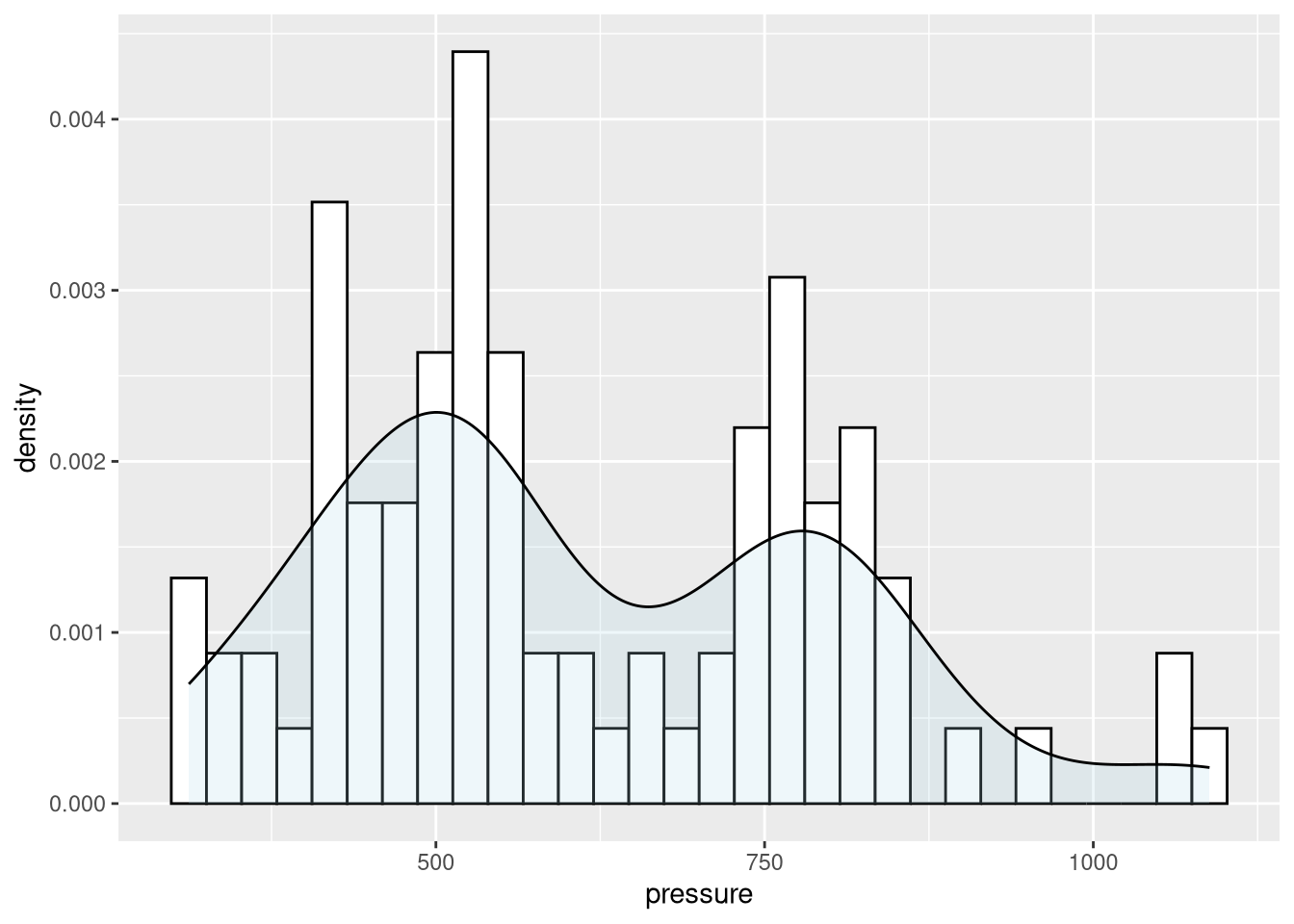
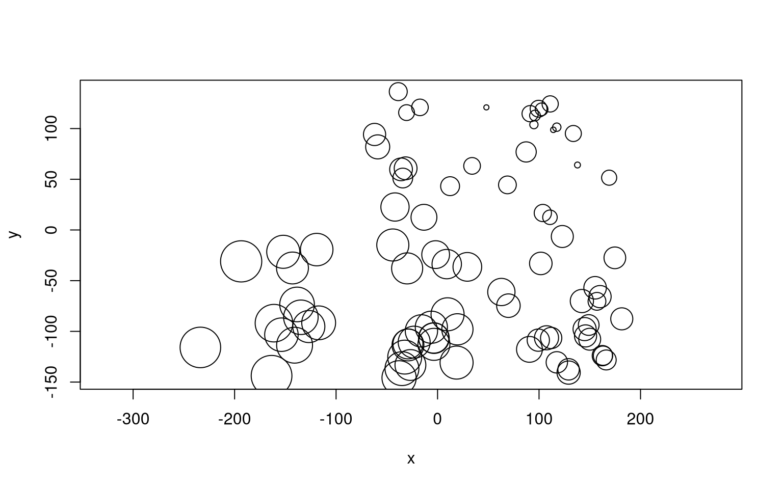
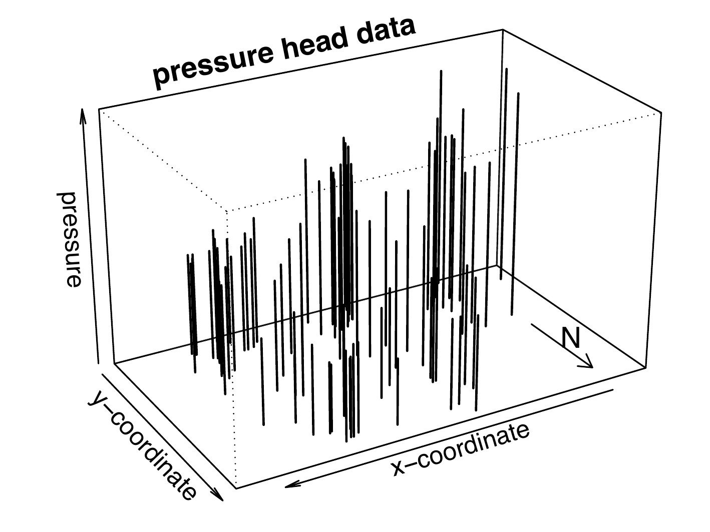
Data on hydraulic head (pressure) in a confined brine aquifer in NW Texas
Hydro-geological study part of evaluation whether region suited to host nuclear waste repository
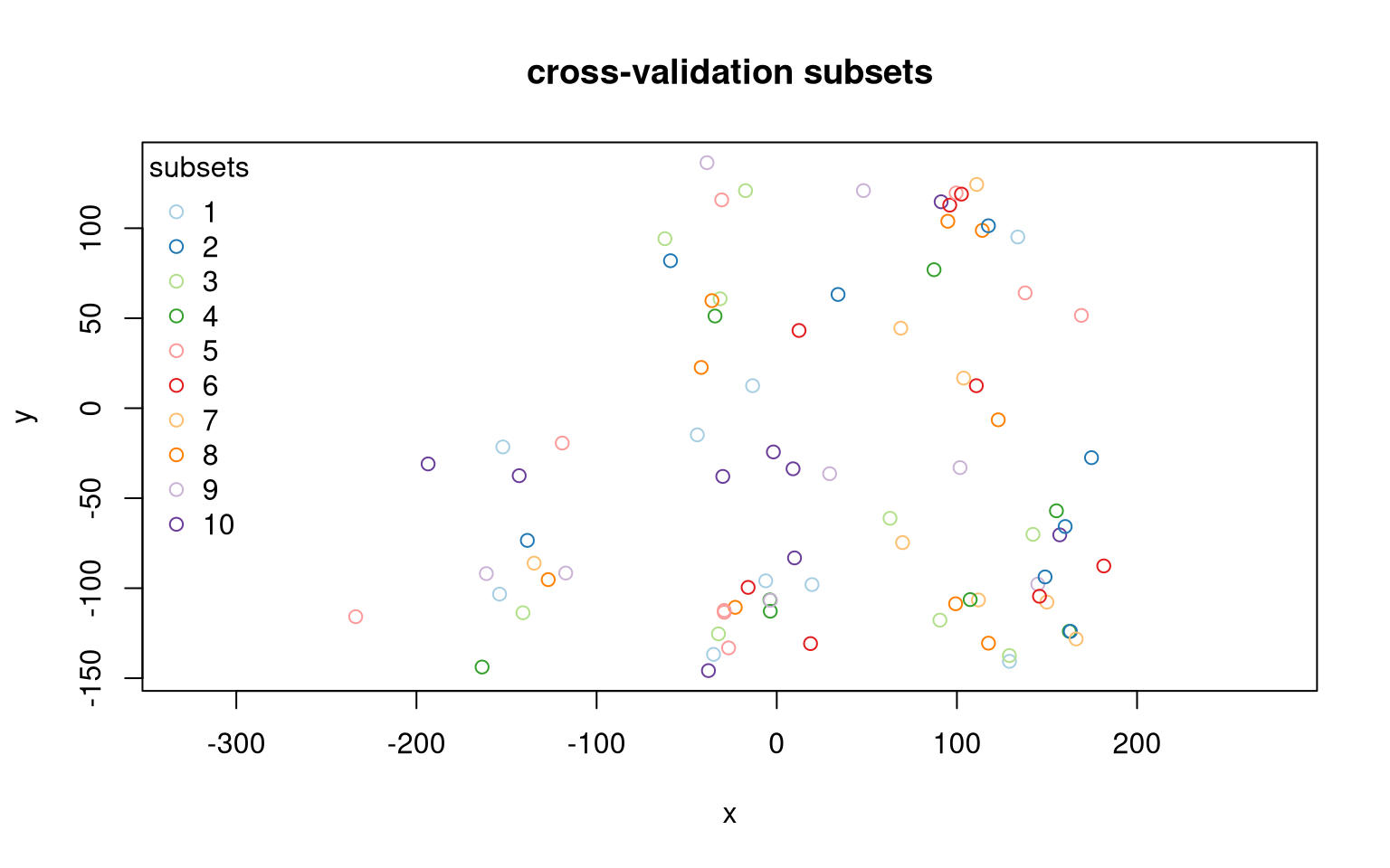
Instead of an non-spatial x-y-plot, we would ideally create a map with a background map to display the locations. However, test datasets have often anonymized coordinates that do not allow for real-world map plotting.
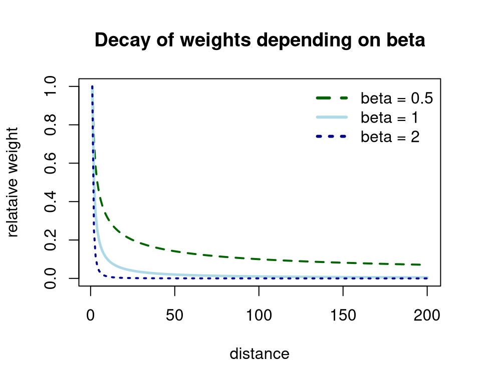
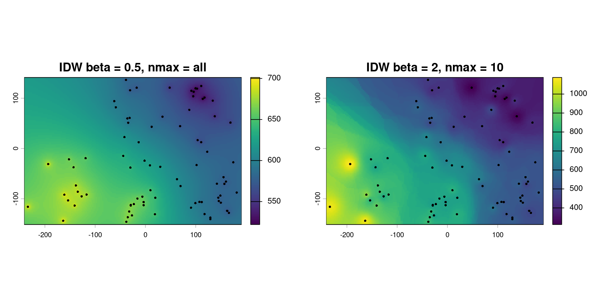
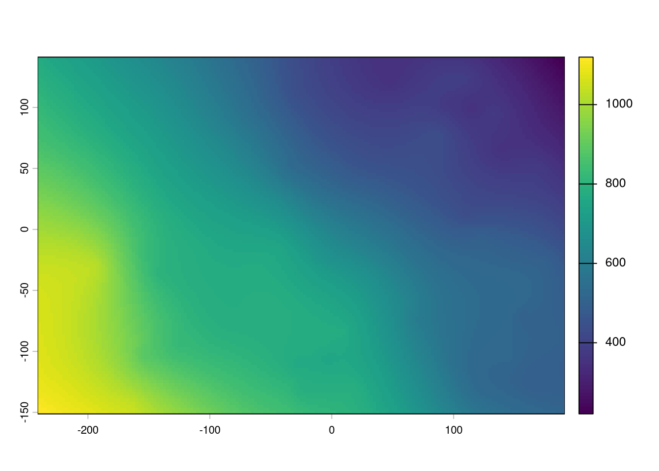
Calculate prediction \(S(\mathbf{x}_0)\) for unsampled location \(x_0\) as weighted mean of the sampling points \(x_i\) with weights \(w(x_i)\) being derived from the pairwise distances \(d(x_p, x_i)\) raised to the power \(\beta\):
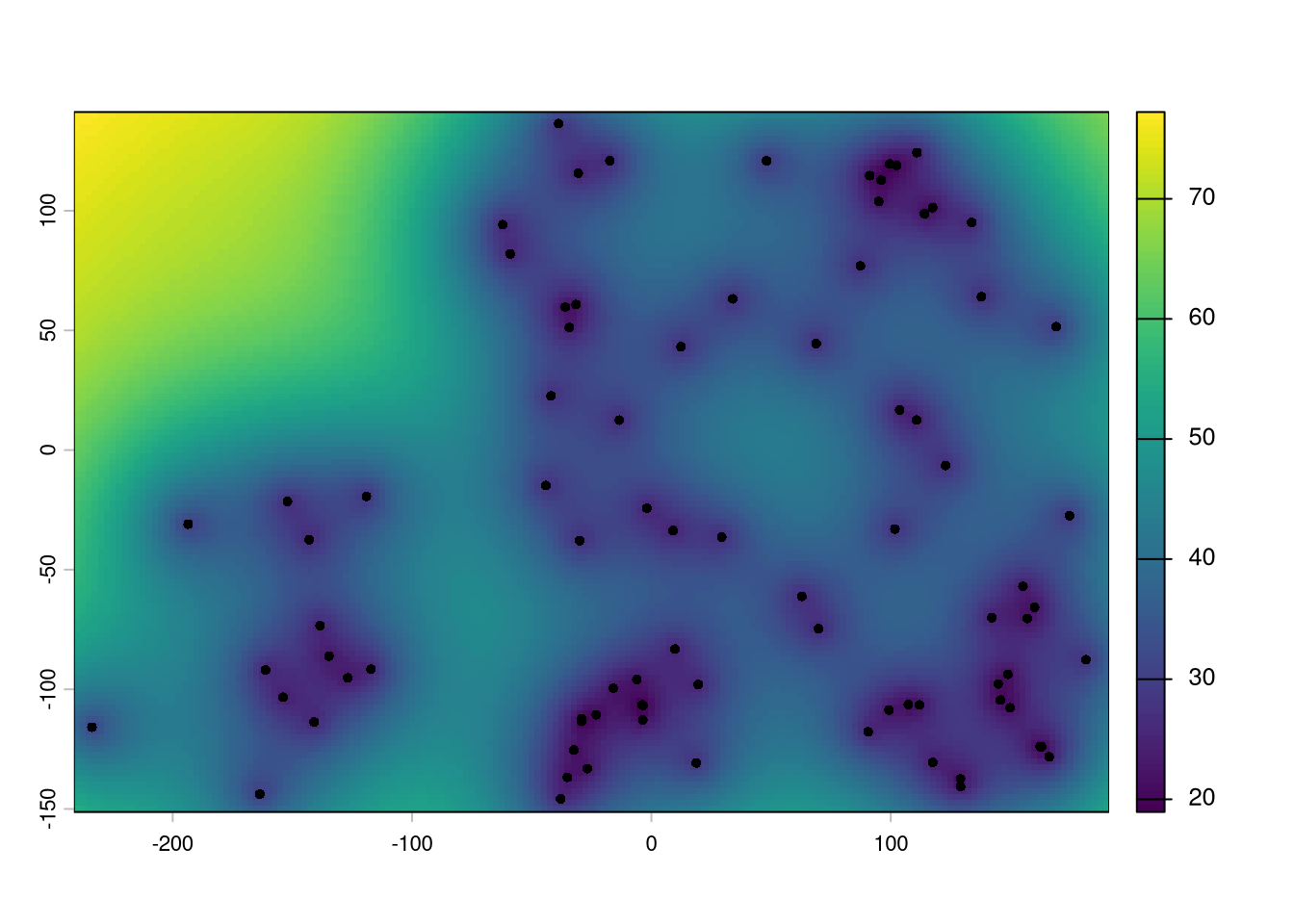
library(gstat)library(terra)idw <-gstat(id ="pressure", formula = pressure ~1, data = d.w, nmax =nrow(d.w), # use all the neighbors locationsset =list(idp =0.5)) # decay of weights by d^0.5# create a regular gridd.w.grid <-expand.grid(x =seq(-240, 190, by=2.5),y =seq(-150, 140, by=2.5))gridded(d.w.grid) <-~x+y# predict for each node of grid d.w.idw <-predict(idw, newdata= d.w.grid)
[inverse distance weighted interpolation]
( d.w.idw <-rast(d.w.idw) )
class       : SpatRaster
size        : 117, 173, 2  (nrow, ncol, nlyr)
resolution  : 2.5, 2.5  (x, y)
extent      : -241.25, 191.25, -151.25, 141.25  (xmin, xmax, ymin, ymax)
coord. ref. :
source(s)   : memory
names       : pressure.pred, pressure.var
min values  :      522.0596,          NaN
max values  :      701.1927,          NaN
Data: measurements \((y_{1,i}, y_{2,i})\), \(i=1,2,\ldots,n\) about 2 response variables
Sample covariance where \(\bar{y}_{1}\) and \(\bar{y}_{2}\) are the (arithmetic) sample means \[
s_{1,2} = \frac{1}{(n-1)} \sum_{i=1}^n (y_{1,i}- \bar{y}_{1}) (y_{2,i}-\bar{y}_{2})
\]
(Pearson) correlation coefficient, where \(s_{1}\) and \(s_{2}\) are the sample standard deviations \[
\hat{\rho} = \frac{s_{1,2}}{s_{1}\; s_{2}}
\]
“plug-in” estimator for auto-correlogram of time series \[
\hat{\rho}(h) = \frac{\sum_{i=1}^{n-h} (y_{i+h} - \bar{y})(y_{i} - \bar{y})}{
\sum_{i=1}^{n} (y_{i} - \bar{y})^2}
\]
The expression is the usual sample autocorrelation function. For a time lag \(h\), it compares observations that are \(h\) time steps apart.
The numerator is essentially a sample covariance between \(Y_t\) and \(Y_{t+h}\): it measures whether values that are \(h\) time steps apart tend to be above or below the mean together. The denominator standardises this by the overall variance, so that the result is a correlation rather than a covariance.
Thus:
\(h=0\): \(\hat\rho(0)=1\)
\(\hat\rho(h)>0\): observations \(h\) time steps apart tend to be similar
\(\hat\rho(h)<0\): observations \(h\) time steps apart tend to be dissimilar
\(\hat\rho(h)\approx0\): little linear dependence at that lag.
Covariance and correlation: visual display
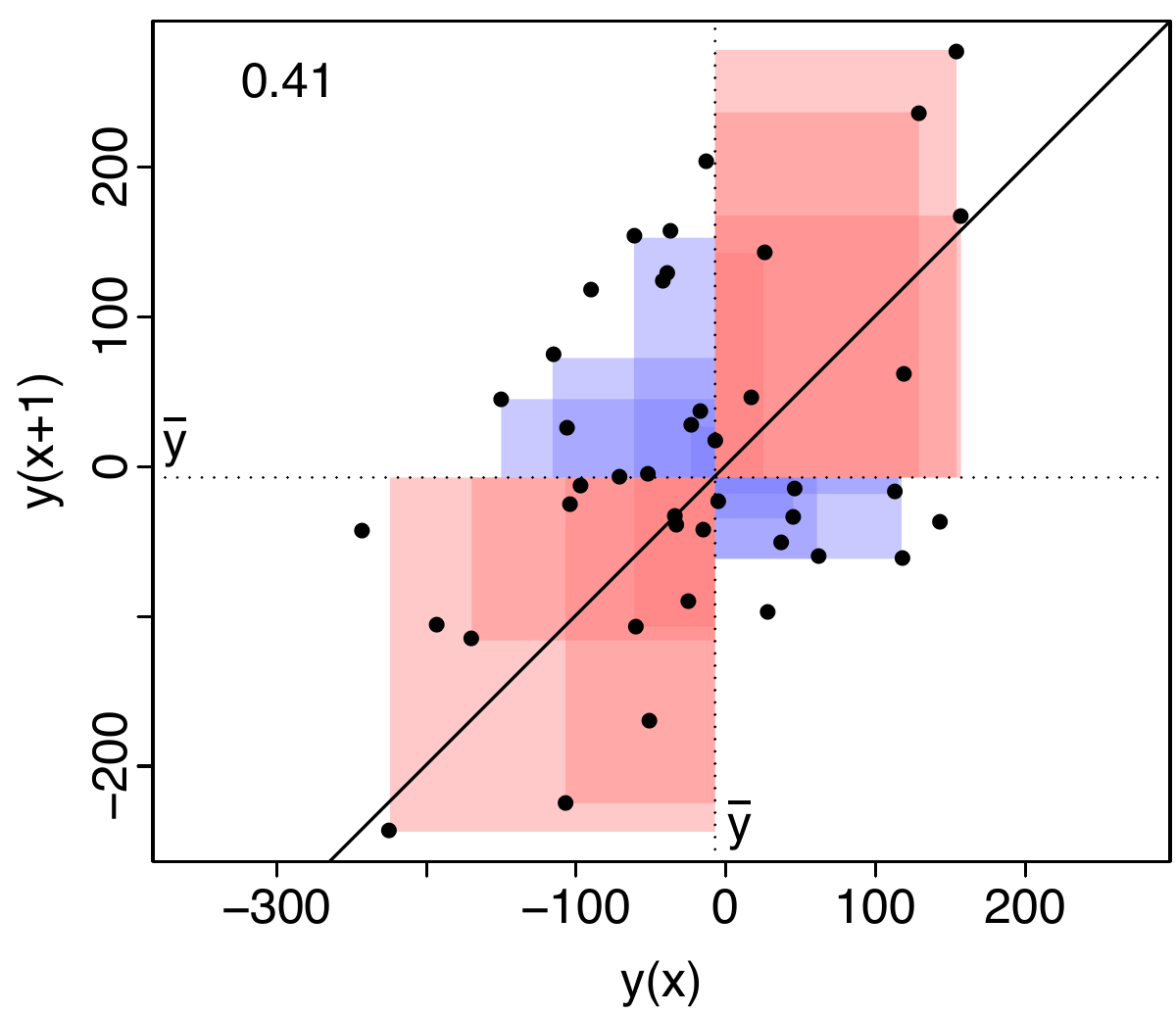
The figure shows a visual display of the covariance of \(y\) at \(x\) and at \(x+1\). The dotted lines correspond to the mean of \(y\). As squares are used this translates to areal features in this figure. Red areas indicate similarity and blue areas dissimilarity. If the red areas are larger, the correlation coefficient becomes positive, if the blue areas are larger, it becomes negative.
Defining lags for irregular sampling grids
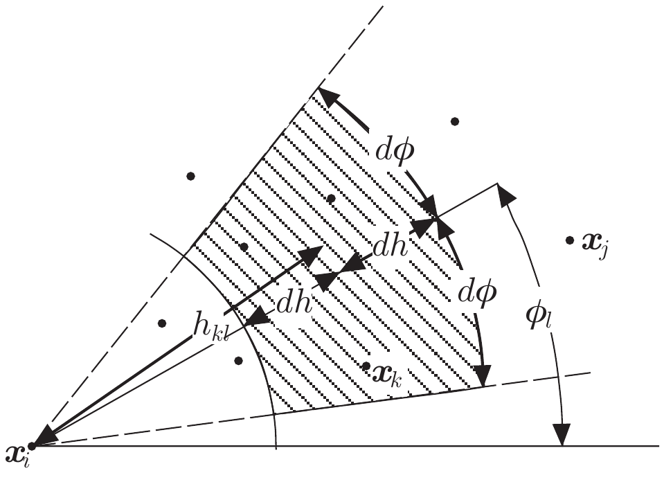
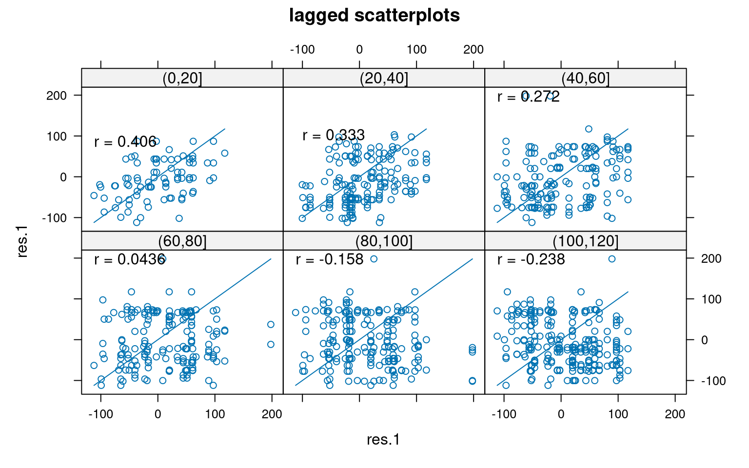
We group pairs of observations according to their spatial lag: their distance and direction. Under isotropy, the direction does not matter. All pairs separated by approximately the same distance contribute to the same variogram estimate.
We can calculate variograms for different directions by restricting the spatial lags to different angular sectors. If the variograms differ between directions, we have evidence of anisotropy.
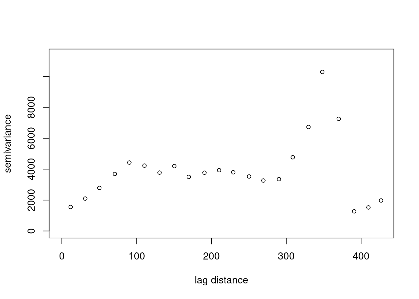
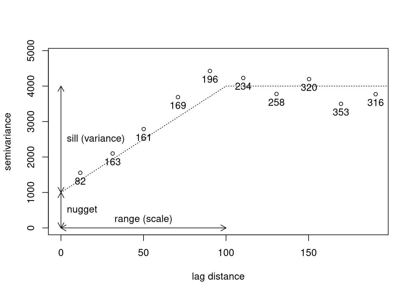
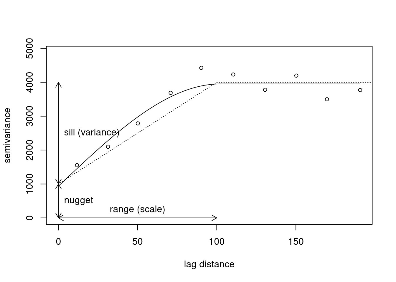
Spatial Auto-correlation: (co-)variogram of spatial data
\((k,l)^{\mathrm{th}}\) lag class, \(\mathbf{h}_{kl}\), characterized by distance, \((h_k-dh, h_k+dh]\), and angular class, \((\phi_l-d\phi,\phi_l+d\phi]\)
\(N_{kl}\): number of pairs of locations \((\mathbf{x}_{i},\mathbf{x}_{j})\) with \(\mathbf{x}_{j} - \mathbf{x}_{i} \approx
\mathbf{h}_{kl}\)
Covariogram: Estimator for covariance for lag class \(\mathbf{h}_{kl}\): \[
\widehat{\gamma}(\mathbf{h}_{kl})=\frac{1}{N_{kl}} \sum_{(i,j) \in
\mathbf{h}_{kl}} [y(\mathbf{x}_{i}) - \bar{y}][y(\mathbf{x}_{j}) -
\bar{y}]
\]
(Semi-)variogram: Estimator for (semi-)variance for lag class \(\mathbf{h}_{kl}\): \[
\widehat{V}(\mathbf{h}_{kl})=\frac{1}{2\,N_{kl}} \sum_{(i,j) \in
\mathbf{h}_{kl}} [y(\mathbf{x}_{i}) - y(\mathbf{x}_{j})]^2
\]
Spatial Auto-correlation: Semi-variance
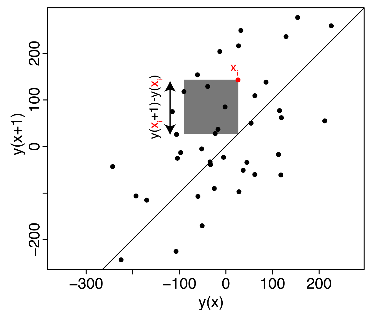
Each point represents a pair of observations separated by the chosen spatial lag (+1). The 1:1 line represents equal values at the two locations. The further a pair lies from this line, the larger the difference between the two values, and hence the larger its contribution to the semivariance.