19 Introduction to Random Forest
Download slides PDF
The PDF contains what was shown during the lecture. Some of these websites include additional text in light gray.
e-Lecture video
This lecture is available as recording.
19.1 Why random forest?
Quite fast model fitting and prediction.
Models interaction in the data, models non-linear relationships and threshold behavior.
Very good predictive power expected, therefore often used for spatial prediction.
No extrapolation over value range of the response.
Prediction uncertainty for continuous responses (at point location).
Not sensitive to user choices or model parameters, easy to implement.
19.2 Random forest - Overview
Ensemble machine learning method
Classification and regression trees (CART) as base element
Bagging (Bootstrap aggregation)
Bagging is a general-purpose procedure for reducing the variance of a statistical learning method.
Large number of trees are fully grown
Trees are decorrelated with
Resampling of original dataset with replacement
Only a random subset of predictors are tested to split tree nodes
Prediction is the average of all trees (continouous response) or the majority vote (binary or multinomial response).
Classification and regression trees – binary splitting
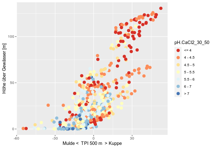
Classification and regression trees – tree
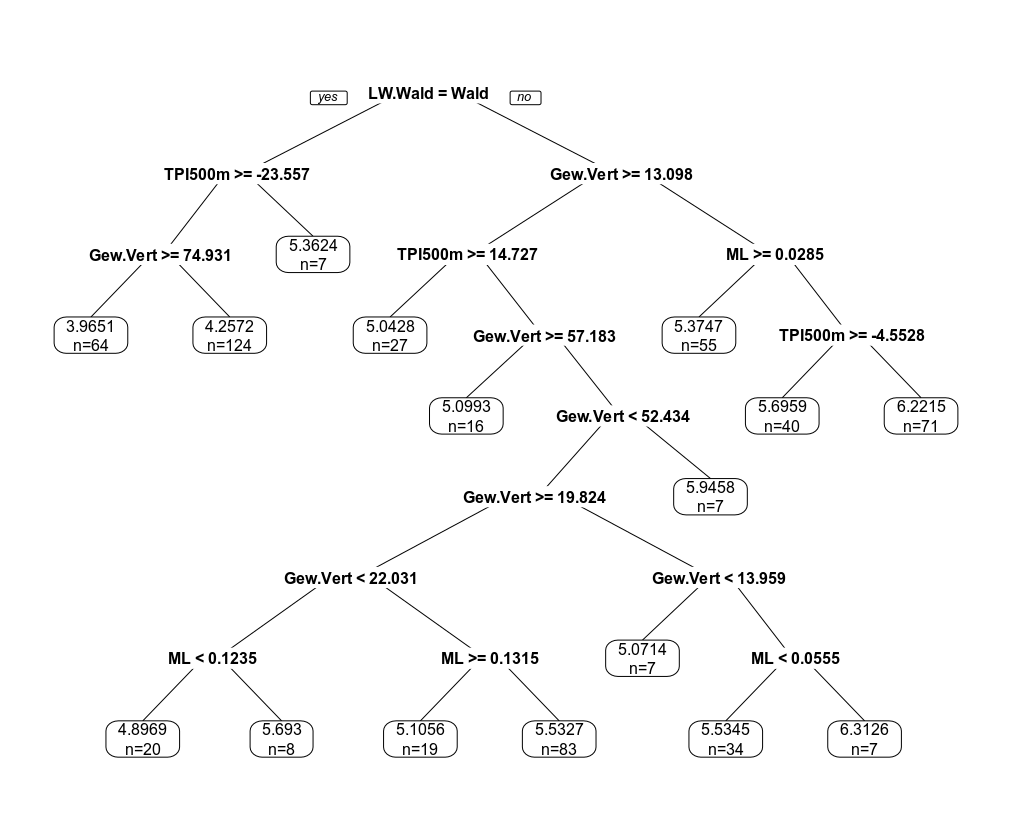
Example regression tree
Response: soil pH
Predictors: forest/no-forest, ML: molasse geological unit, topographic index, vertical distance above river.
Value in box: mean pH of all locations falling in this tree node.
Classification and regression trees – formally
Technique: Recursive binary splitting
Consider all predictors \(X_1, ... , X_p\), and all possible values \(s\) for splitting for each of the predictors, and then choose a predictor \(X_j\) and splitpoint \(s\) such that the resulting tree has the lowest residual sum of squares.
For any \(j\) and \(s\) a half-plane is defined by \[ R_1(j,s) = \{X|X_j<s\} ~~~\text{and}~~~ R_2(j,s) = \{X|X_j \geq s\} \]
where \(j\) and \(s\) are chosen to minimize
\[ \sum_{i: x_i \in R_1(j,s)}(y_i - \overline{y}_{R_1})^2 + \sum_{i: x_i \in R_2(j,s)}(y_i - \overline{y}_{R_2})^2 \]
with \(\overline{y}_{R_1}\) and \(\overline{y}_{R_2}\) being the mean of the observations values in tree node \(R_1(j,s)\) and \(R_2(j,s)\), respectively.
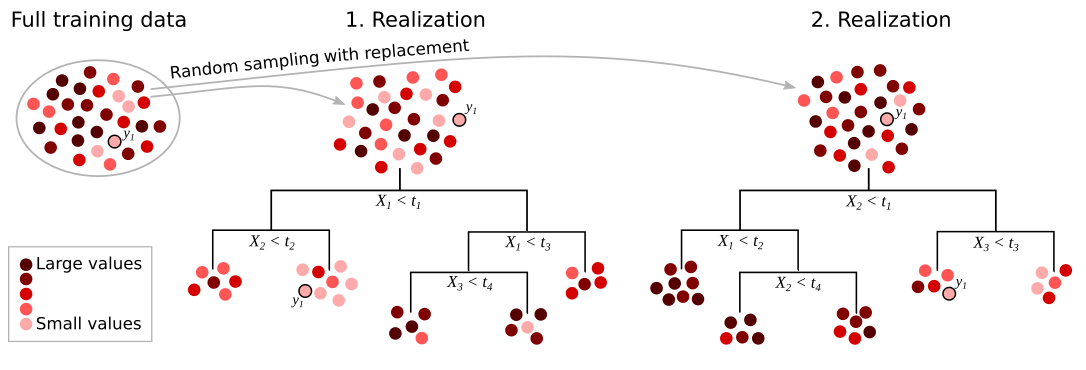
Random forest algorithm
Resample dataset (with replacement)
Take a random sample of predictors of size
mtryTest all selected predictors: find optimal predictors value to split data into 2 portions
Chose predictors with lowest error (e.g. MSE) and split data
Continue to split the data with (3)-(4) until you are left with a small number of data points (
min.node.size) in each leaf of the treeRepeat (1)-(5)
ntreetimes
Random forest tuning
Main tuning parameters:
mtry: number of randomly selected predictors to test at each splitntree: number of trees (mostly not sensitive, if large enough)min.node.size: size of remaining dataset in tree leaf, when it stops to split (mostly not sensitive, if small enough)
Other options:
splitrule: loss function to split datamax.depth: limit tree depth (interaction depth), otherwise fully growncase.weights: increase/decrease weights of to be sampled for a tree (e.g. because of data quality)… many more (in general not changing the big picture)
The naming of model parameters in this section is based on the R package ranger. Other packages, e.g. also in python, allow mostly for the same parameters to be tuned, but naming is different.
Since the observations are chosen randomly for each tree and the predictors are chosen randomly to test, random forest implements bootstrapping on both rows and columns of the design matrix.
In original algorithm (Breimann, 2001) classification or regression trees are fully grown. Moreover, bootstrap is always done. Sometimes examples suggest to tune the tree depth and if the bootstrap resampling of the observations should be done. Not fully grown trees or no bootstrapping will likely result in less stable prediction.
Random forest – Default objective function
Regression – Mean squared error
\[ MSE = \frac{1}{n} \sum_{i=1}^n (y_i - \hat{f}(x_i))^2 \]
with \(y_i\) being the observed value, \(\hat{f}(x_i)\) the prediction that prediction function \(\hat{f}\) gives for the \(i\)th observation and \(n\) the total number of observations. For random forest, \(\hat{f}\) is the mean prediction of all fitted regression trees.
Classification – Gini index \[ G = \sum_{k=1}^K \hat{p}_{mk}(1-\hat{p}_{mk}) \]
with \(\hat{p}_{mk}\) being the proportion of training observations in the \(m\)th tree leaf from the \(k\)th class (response category), across all \(K\) classes.
Random forest – Compute predictions
CART
For each location, decide in which tree end node it falls (“send” each location with its predictor values down the trees). Take the mean (regression) or proportion/majority class (classification) of the observations within this end node.
Random forest
With \(\hat{f}^1(x), \hat{f}^2(x), ..., \hat{f}^B(x)\) being predictions of one single CART, random forest predictions are averaged over \(B\) different bootstraped (bagged) samples \(b\) used for the training of \(\hat{f}^b(x)\)
\[ \hat{f}_{bag}(x) = \frac{1}{B} \sum_{b=1}^B \hat{f}^b(x). \]
For regression, this results in a weighted mean of all the observations. For classification, we obtain proportion of classes “voting” for an categorical outcome.
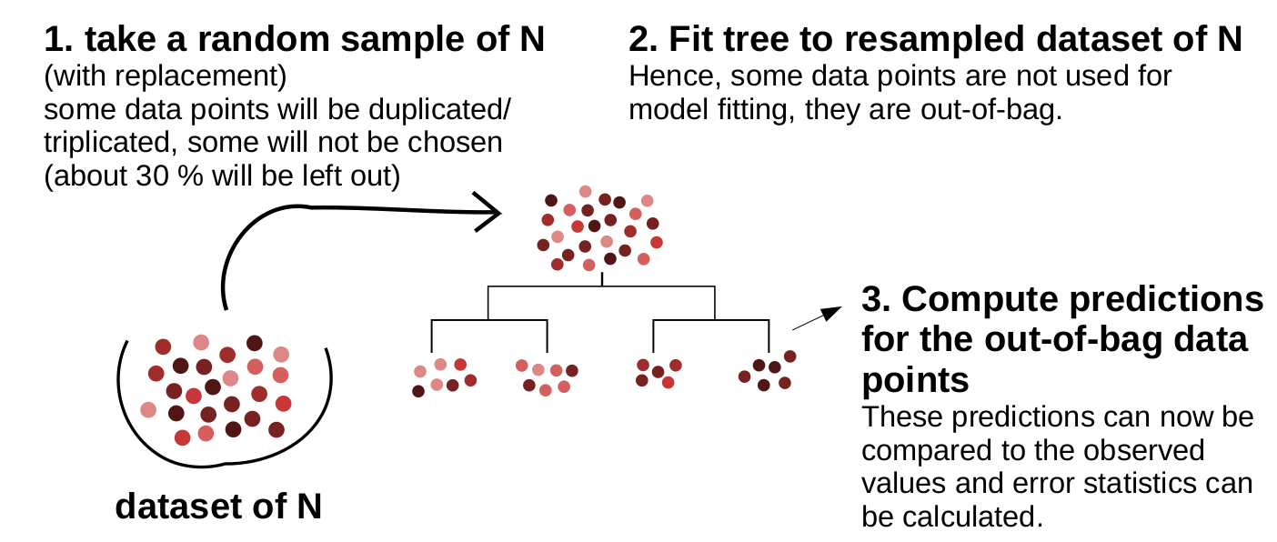
Random forest – Out-of-bag predictions
- Due to resampling with replacement, ~1/3 of observations is not used for one single tree. They are “out-of-bag” (OOB).
Predict the response for the \(i\)th observation using each of the trees in which that observation was OOB.
To obtain a single prediction for the \(i\)th observation, average these predicted responses (regression) or take majority vote (classification). This leads to a single OOB prediction for the \(i\)th observation.
This bootstrap procedure is roughly equivalent to cross-validation.
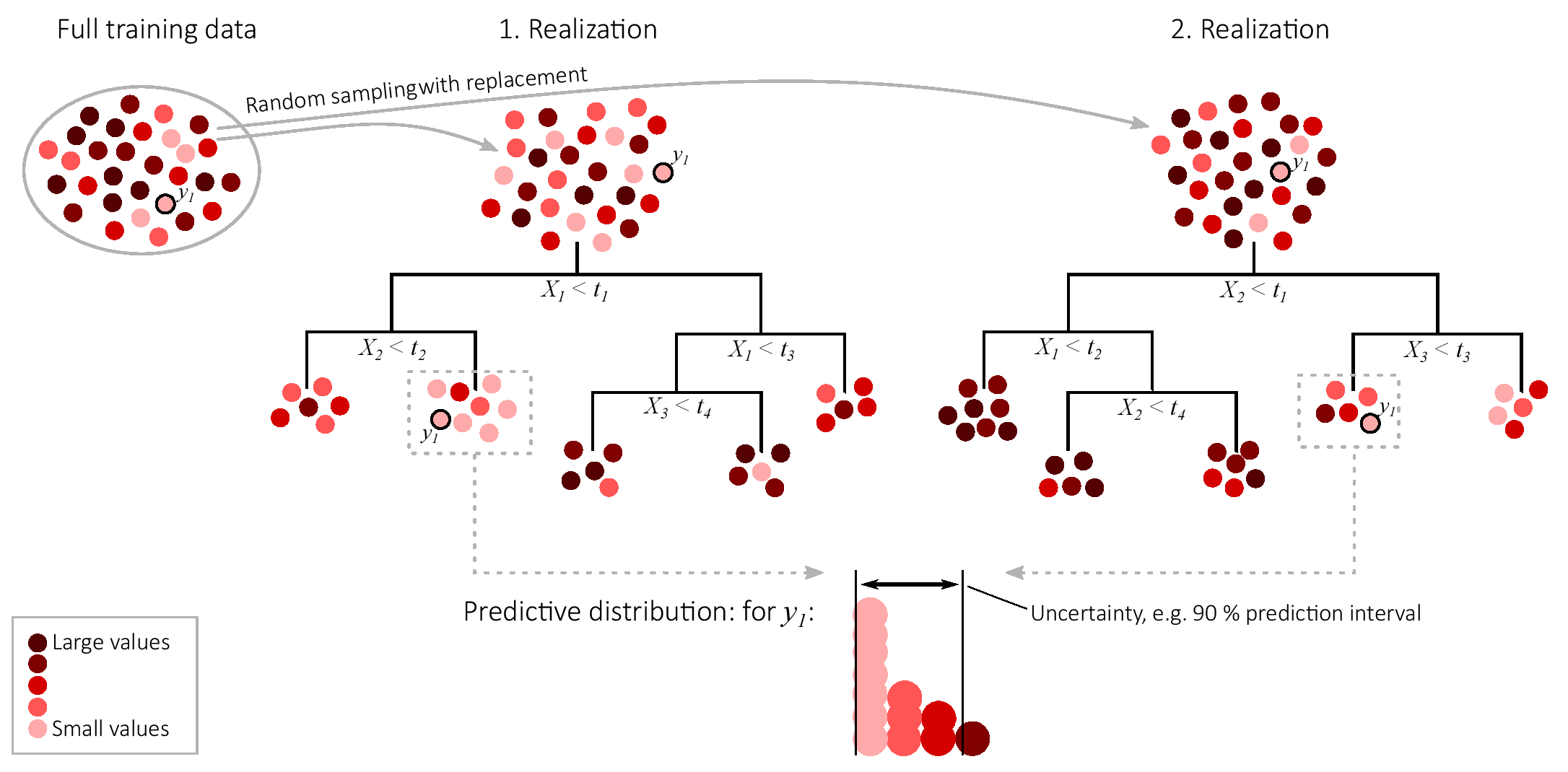
19.3 Quantile regression forest – Uncertainty
Keep all observations in the final tree leaves
Get distribution \(D\) from all observations that were in tree leaf with observation \(y_i\)
Compute required quantities from \(D\) like 90 % prediction intervals or standard errors
19.4 Random forest - summary
- Bootstrap aggregation method
- Uses classification or regression trees
- Adds some more randomness to the trees to make them more dissimilar
- Predictions are the mean of all trees, i.e. the data points in the tree leaves → cannot extrapolate beyond value range
- Often not sensitive to outliers
- Widespread use, especially for medium-sized datasets