27 Sampling for ML and validation
Download slides PDF
e-Lecture 1. part video
Where would you select sampling points manually?
Download Handout PDF
e-Lecture 2. part video
This lecture is available as recording.
Lecture overview
Short introduction into sampling designs for training of machine learning models and map accuracy assessment.
Digital soil mapping
Sampling for soil mapping
Computer practical:
Sampling for model training to create a soil map
Sampling for map validation
Do the sampling (virtually) and create a map
27.1 Sampling for soil mapping
Need for soil information
Soil data or information: maps, point observations, monitoring networks.
Needed by many actors like governments, companies, farms:
- Local applications: prevent soil compaction, subsidies to prevent erosion
- Spatial planning: save high-quality soils for agriculture and plan nature reserves at locations with high habitat potential
- Monitor soil health on European level
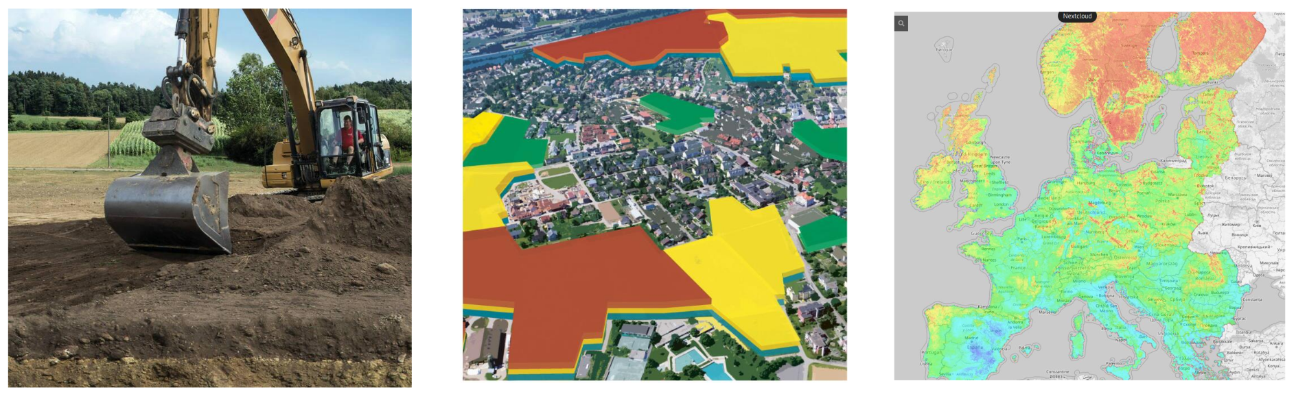
Example: Soil depth determines agricultural use


Soil forming factors
Factors influencing soil formation:
Parent material, terrain, climate, organism including humans, time.
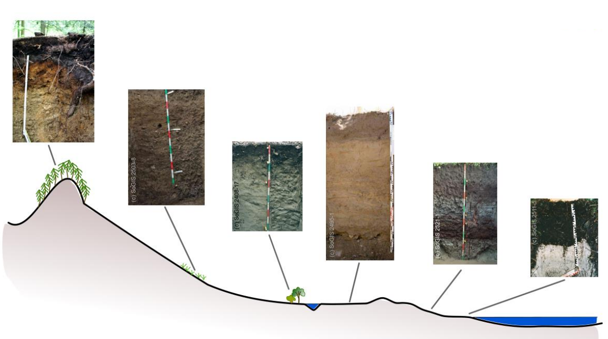
Digital soil mapping
Commonly used approach: geostatistical prediction/interpolation, from point observations to continuous raster.
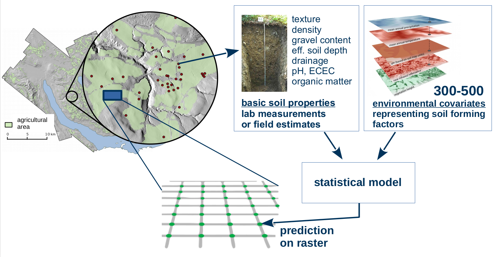
Digital soil mapping
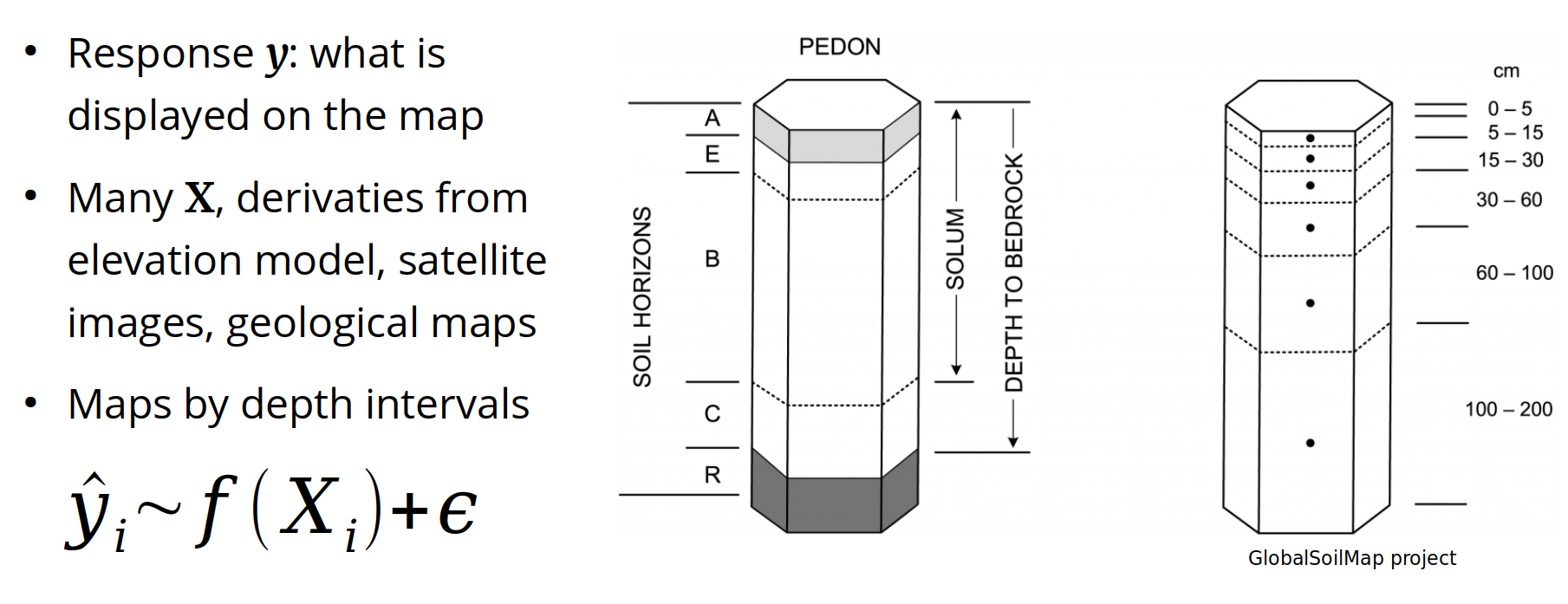
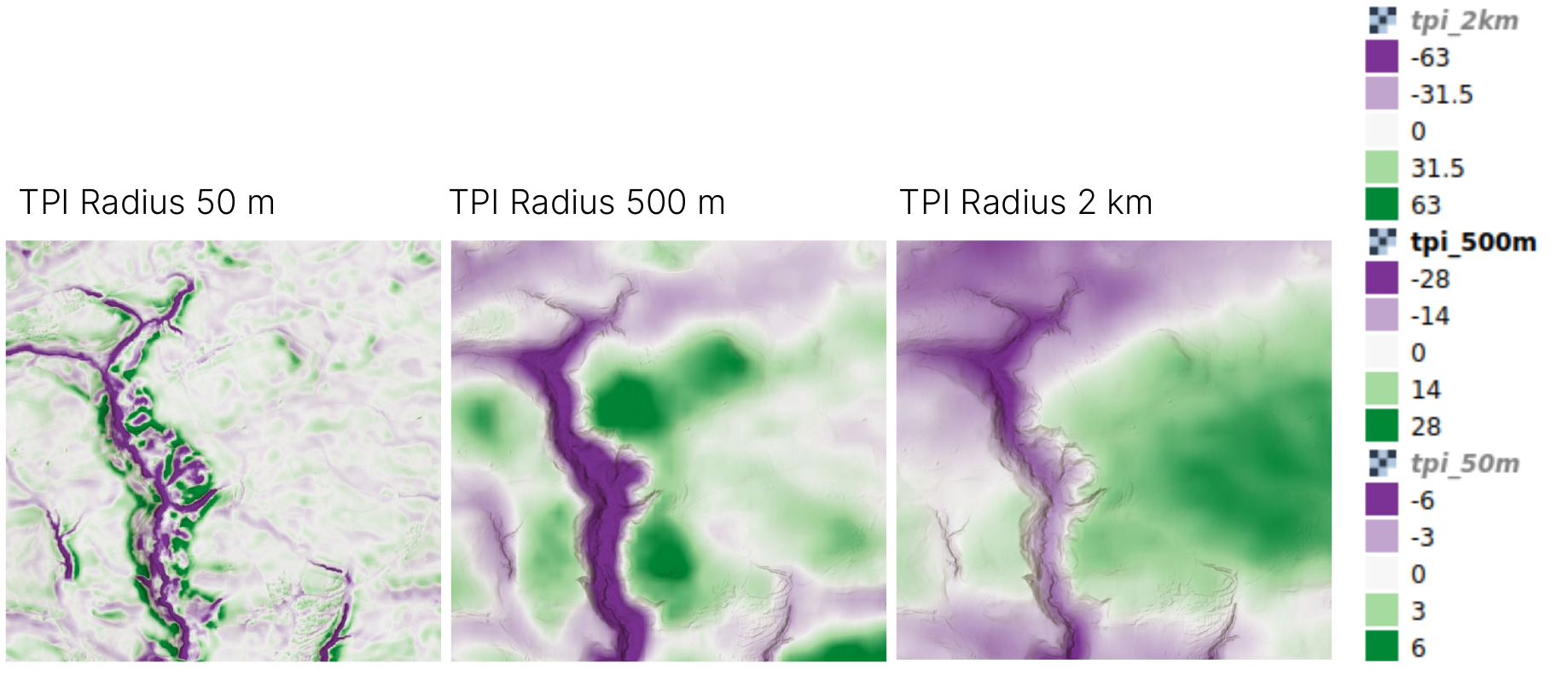
Example predictors: Terrain attributes
Topographic position index, identifying valleys and hilltops at multiple scales.
What samples do we use?
Common situation:
Use what is there and do our best …
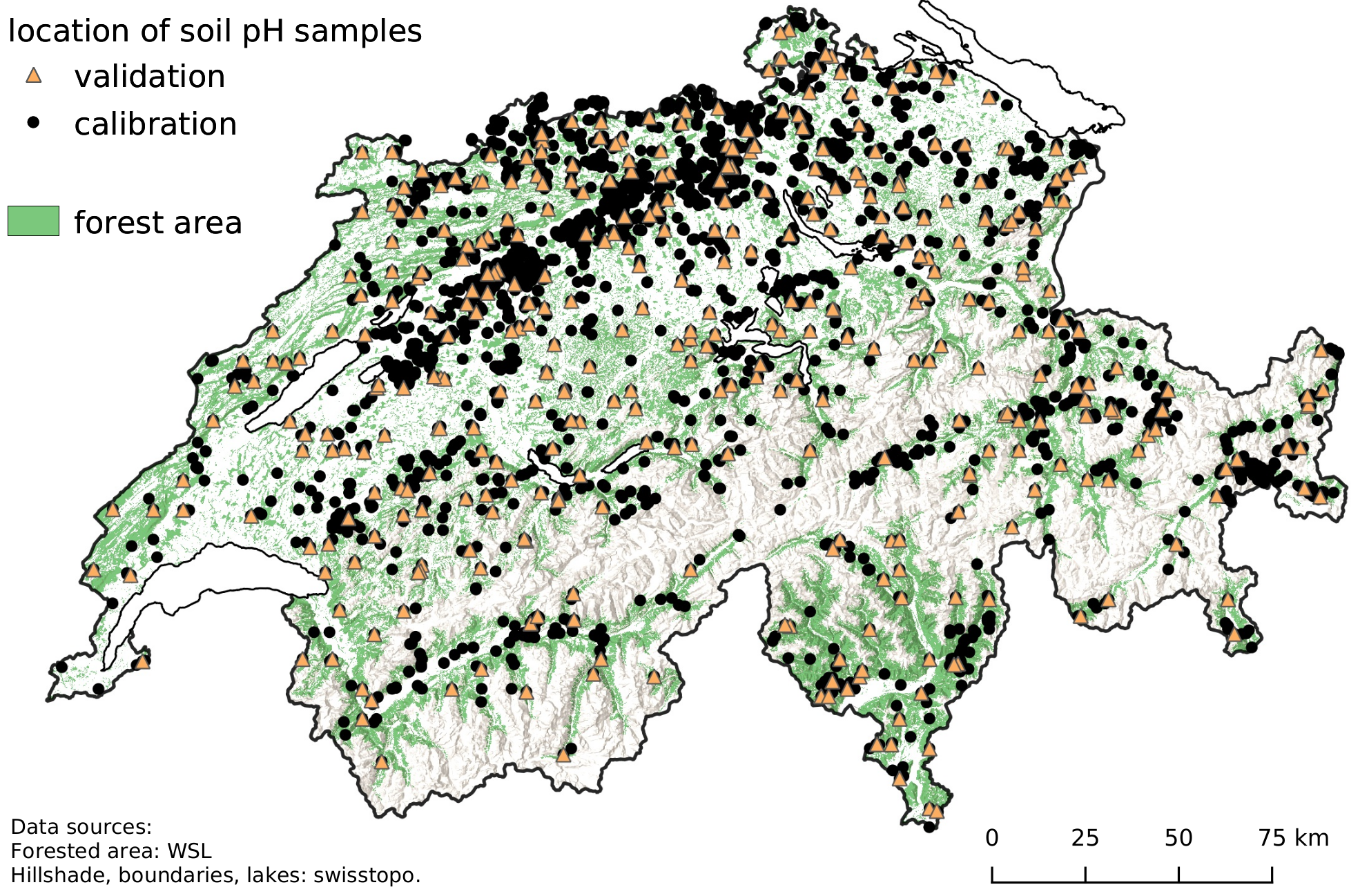
Example: maps for forested area of Switzerland
Example: Mapping of soil properties (e.g. pH, soil organic carbon content, clay content) for forested area of Switzerland.
Goal: model scenarios of tree species under climate change.
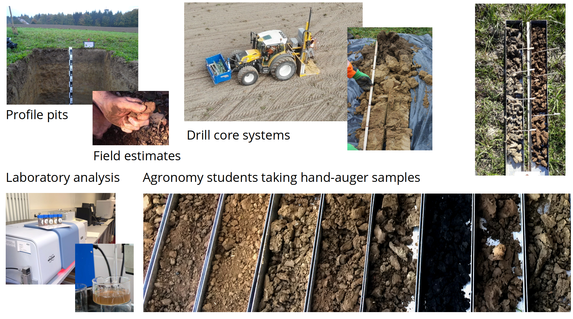
New sampling: what does that mean
New sampling: where to go?
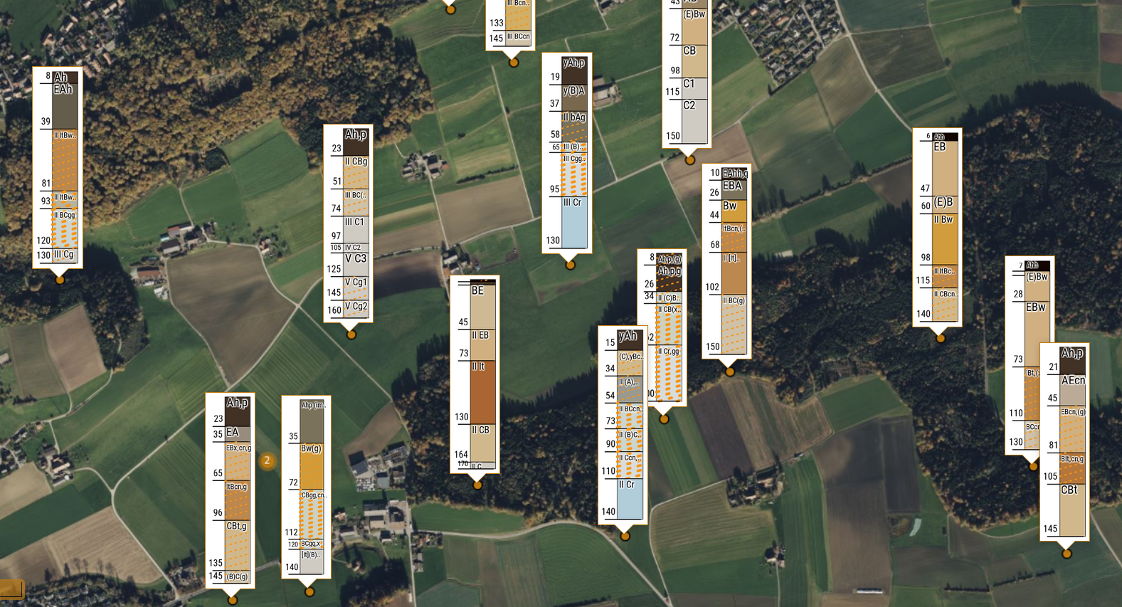
Result based on new survey
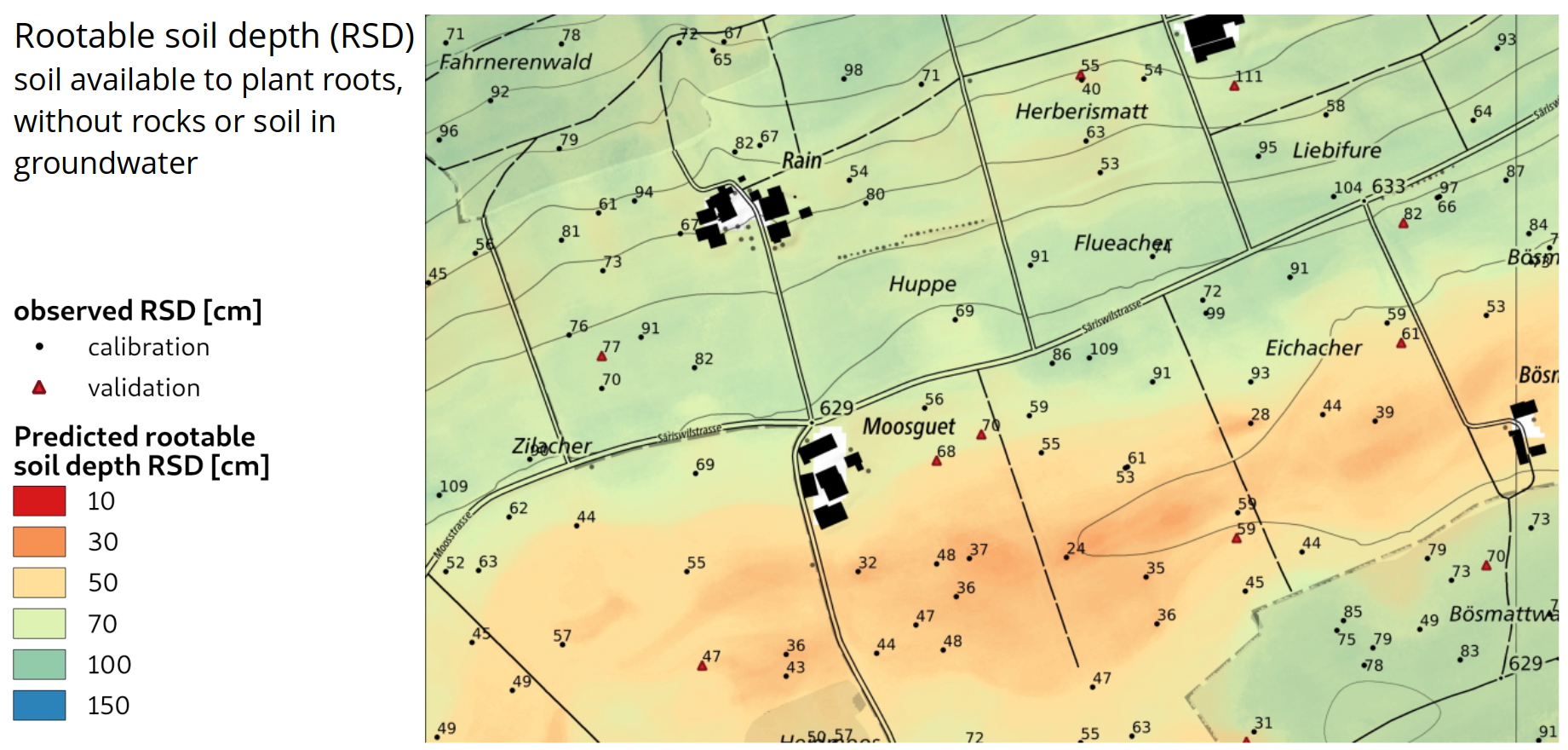
27.2 Manual selection of locations
How would you place samples?
Example study area:
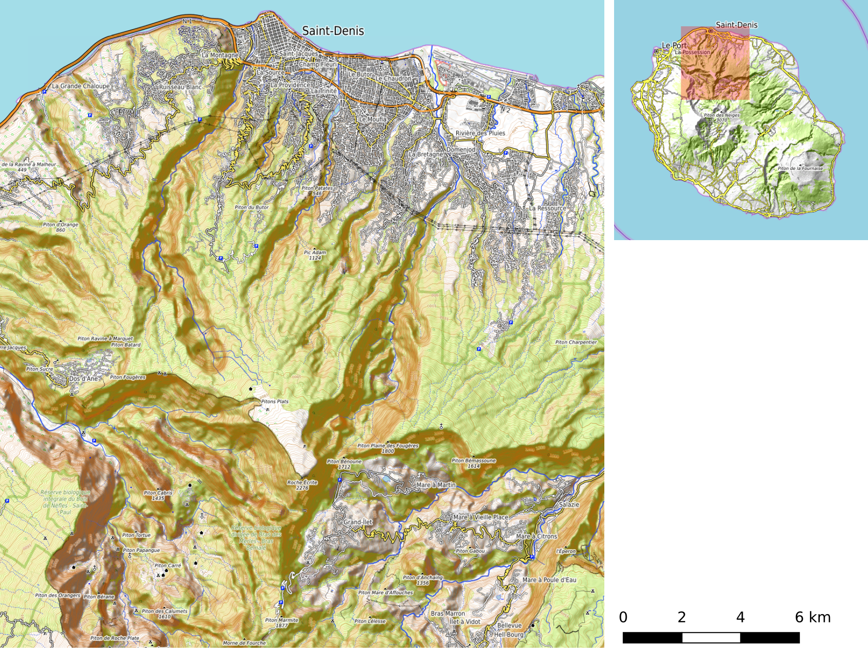
La Réunion
Goal: Create a topsoil organic carbon map.
Task: Draw locations where you would sample.
10 locations for model training (cross)
5 locations for model validation (triangle)
27.3 Spatial sampling: some theory
Large number of sampling approaches
Sampling: always regarding a specific goal.
No sampling design is optimal for all cases, but we can combine different goals (e.g. in model-assisted sampling)
Some possible approaches:
- Random sampling: Simple or stratified random sampling
- Systematic sampling: Regular grid sampling
- Nested sampling: Main locations with sublocations
- Targeted sampling: e.g. for finding pollution or rare species
- Sampling for monitoring: repeated measures
- Geostatistical sampling: optimal for variogram estimation
- Model based sampling for model training
Design-based vs. Model-based Sampling
Design-based Sampling
- Definition: Randomness ensures unbiased estimation
- Key Idea: Each unit has a known, non-zero probability of being sampled.
- Assumptions: No model assumptions; inference is based on probability theory.
- Example: Simple Random Sampling (SRS), Stratified Sampling.
Model-based Sampling
- Definition: Assumes an underlying model for the population.
- Key Idea: The inference is based on the assumed model rather than sampling probabilities.
- Assumptions: Requires a correctly specified model.
- Example: Sampling based on variogram (kriging), regression-based estimation or prediction.
27.4 Coverage sampling for training
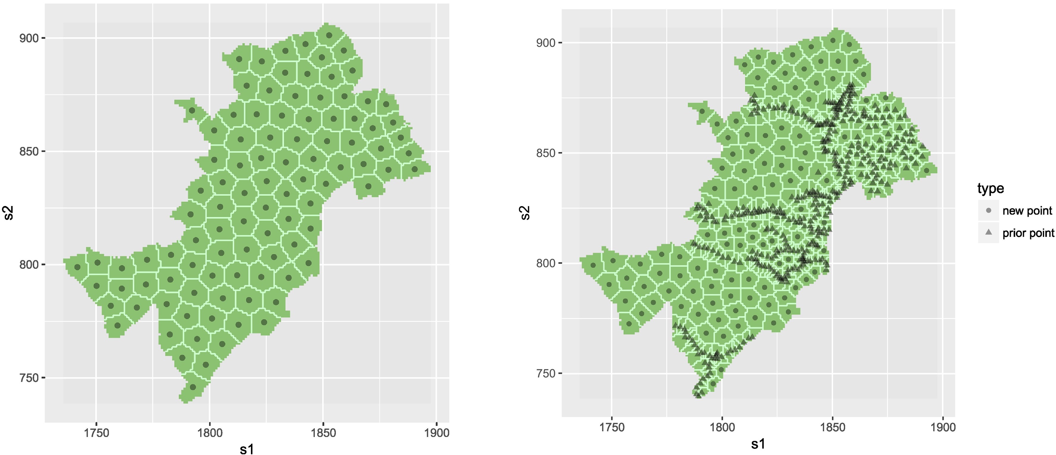
Spatial coverage sampling for model training
Apply k-means clustering to spatial coordinates.
Sampling for calibration of linear regression
Ideal case: univariate linear dependence with known minimum and maximum.
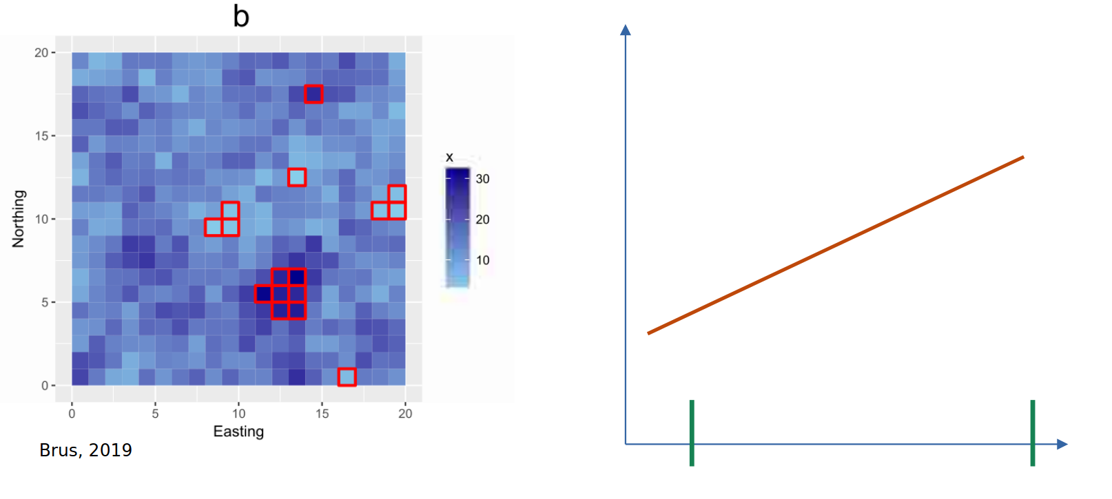
Coverage over predictors
Feature space coverage sampling design
Apply clustering method to all candidate sampling locations.
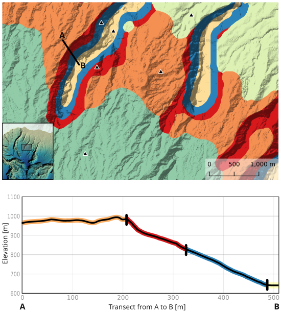
Variables for clustering: most important predictors (here elevation, slope, TPI 1500 m).
Replacement: move within same cluster.
27.5 Probability sampling for validation
Validation of map quality
Goal: estimation of average map error = estimation of a population parameter
Recommended approach: Stratified random sampling.
Strata: sub-units with more homogenouous distribution of errors
Compared to simple random sampling: more accurate estimates with the same number of samples.
Replacement samples: if a location is not accessible, another random location needs to be sampled (even if it is faraway).
Horvitz-Thompson Estimator
Purpose: Unbiased estimator for population parameters when inclusion probabilities are not the same for every point (number of samples not proportional to area).
Formula for stratified random sampling over all strata (see p. 51, Brus, 2022) \[ \hat{\bar{z}} = \frac{1}{N}\sum_{h=1}^H\sum_{k \in S} \frac{1}{\pi_k}z_k \] where:
\(\hat{\bar{z}}\) unbiased mean parameter estimate.
\(z_k\) is the observed value for sample \(k\).
\(\pi_k\) is the inclusion probability of sample \(k\), for each stratum are \(\pi_k = \frac{n_h}{N_h}\) for all \(k\) in stratum \(h\) with \(n\) the sample size of stratum \(h\) and \(N_h\) the size of the stratum.
\(S\) is the sample for stratum \(h\).
Note: With equal sample sizes per stratum the formula can be simplified to a weighted mean of the stratum means, with weights \(w_k = N_h/N\).
Example
Suppose we sample 2 samples from three areas (strata) with size 200, 500 and 400 km\(^2\). To compute inclusion probability we consider each 1 x 1 km grid node as finite sample candidates (total \(N =1100\)).
For our example \(\pi_1 = 0.01\), \(\pi_2 = 0.004\), and \(\pi_3 = 0.005\). Their corresponding observed values are (2,3), (4,5) and (6,7).
The estimator correcting for unequal stratum size is: \[ \hat{\bar{z}} = \frac{1}{1100} \left( \frac{2}{0.01} + \frac{3}{0.01} + \frac{4}{0.004} + \frac{5}{0.004} + \frac{6}{0.005} + \frac{7}{0.005} \right) = 4.863. \]
As opposed to the unweighted mean = 4.5