22 Predictor selection and interpretation
Download slides PDF
The PDF contains what was shown during the lecture. Some of these websites include additional text in light gray.
e-Lecture video
This lecture is available as recording.
22.1 Select relevant predictors
Model building
Select structure of the model, i.e. relevant predictors and relevant response-predictors relationships.
Model selection
Select relevant predictors, drop non-relevant or correlated predictors
Model selection – reasoning
Model selection, why:
Decrease computing time (e.g. for prediction).
More insight what is important. Improve future predictor preparation.
Large number of strongly correlated/nearly identical predictors might lead to overfitting.
Why not:
Potential loss of predictive performance.
Chosen ML algorithm should be able to deal with large number of correlated predictors
Correlated predictors might improve predictions locally, at tail of distributions.
Control overfitting by method (e.g. bagging, regularization).
Removal of many predictors might lead to jumpy/uneven final map.
Model selection with random forest
Variable importance
2 types of predictor importance:
Sum of decrease in goodness-of-fit error by adding splits of this predictor (impurity), oriented on fitting the data. How much do we reduce error by using this predictor at this split?
Mean decrease in OOB error by randomly permuting a predictor, oriented on predictions. How much worse do OOB predictions get if we randomly shuffle a predictor?
→ removing a predictor is not the same, other correlated predictor could replace its “predictive capacity”
22.2 Approach 1: Recursive backward elimination
Remove predictor(s) with lowest importance.
Refit random forest with remaining.
Repeat (1)-(2) until all predictors are removed.
Find optimum number of predictors with minimal OOB error.
Recursive backward elimination often results in very strong removal of predictors. Resulting maps are not smooth any longer, i.e. tree based predictions become “jumpy”.
22.3 Approach 2: Boruta algorithm
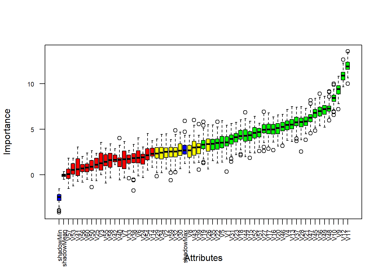
All predictors are shuffled randomly. Shuffled predictors are appended to original predictors (shadow predictors).
Refit random forest with “real” and “shadow” predictors
Repeat (1)-(2) multiple times with different random seed.
Keep only predictors that are on average of larger importance than the shadow predictors.
Boruta algorithm result
blue: shadow predictors, minimum, mean, maximum
green: larger importance than shadows
yellow: unclear decision (within variation of shadow max)
red: smaller importance than shadows
22.4 Model interpretation - Effects plots
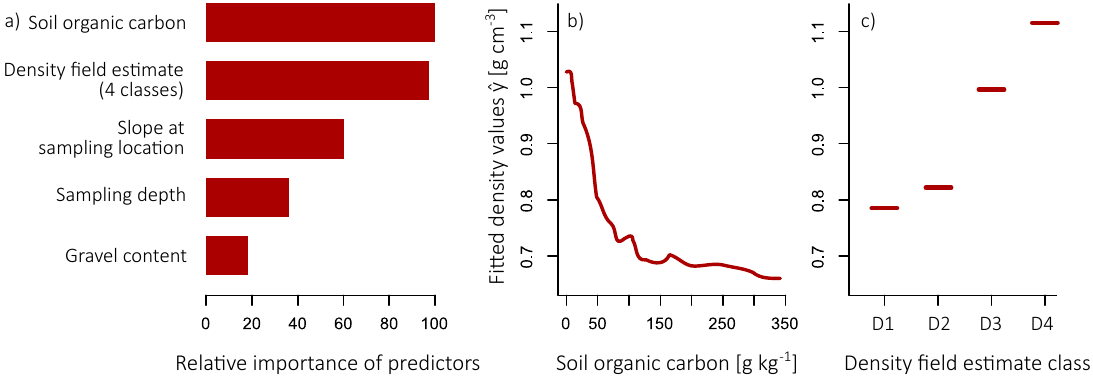
Partial dependence plots
Partial depencende function \(\hat{f}_s\) for the predictor \(s\) evaluated by calculating averages over the data used for model calibration:
\[ \hat{f}_s(x_s) = \frac{1}{n} \sum_{i=1}^n \hat{f}(x_s, x_C^{(i)}) \]
Partial dependece function reports for given value of predictor \(s\) the average marginal effect on the prediction. \(x_C^{(i)}\) are actual predictor values for remaining predictors in which we are not interested in. \(n\) is the number of observations in the dataset.
Assumption: no correlation between predictor \(s\) and remaining predictors \(C\).
Partial dependence plots – example
Accumulated local effects plots
Accounting for correlation structure in predictors.
Instead of using mean of remaining predictors \(x_C\) a moving window approach is implemented.
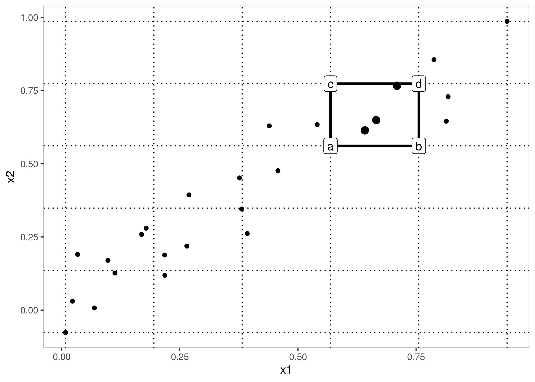
Accumulated local effects plots – example
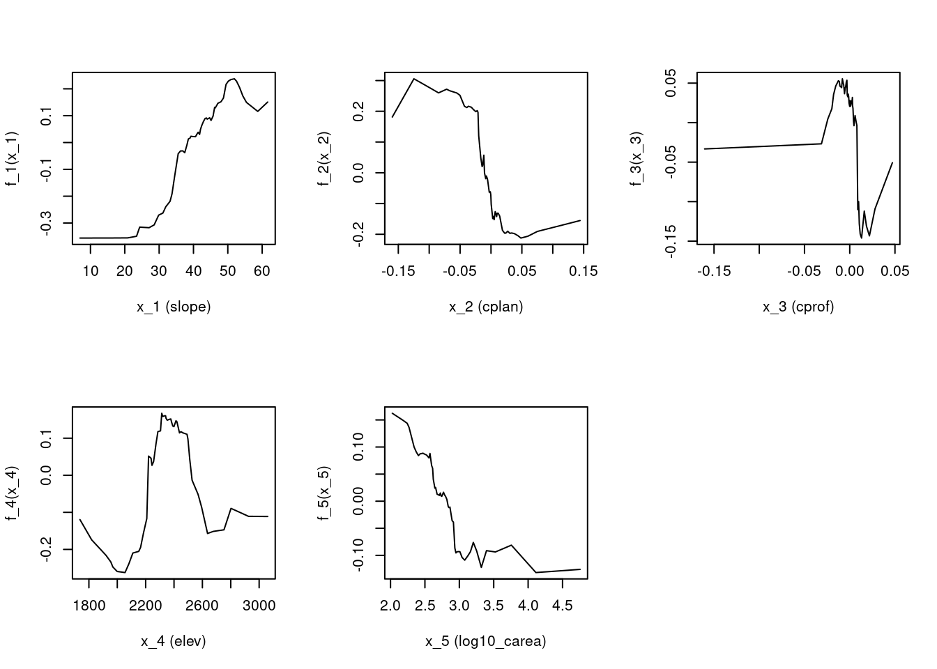
Accumulated local effects plots of the landslide classification example in the computer practical.
Model selection & Interpretation – conclusions
Machine learning can deal with large numbers of predictors.
We might still want to remove the non-relevant predictors, to make models simpler and computations faster.
Machine learning is not just “black box”. We can apply procedures to extract relationships.
Such relationships are however often difficult to interpret, because they are purely correlation based.
The extracted relationships only reflect the underlying process, if the correlations are present in the data. This is not the case if
- there are large errors in the data (e.g. measurement error),
- we have very complex processes and only have few data points,
- we use proxy-predictors that are rather showing pseudo-correlation (e.g. NDVI from satellite images instead of tree stem diameter to estimate biomass).