20 Spatial correlation in RF
Download slides PDF
The PDF contains what was shown during the lecture. Some of these websites include additional text in light gray.
e-Lecture video
This lecture is available as recording.
20.1 Machine learning for spatial prediction
Advantages
Machine learning (ML) handles today’s requirements well
Large dataset sizes (n observations, n covariates)
Lowering computational demands
Automatic model selection and building of model structure
Non-linear models, relaxed model assumptions (non-Gaussian)
Classification tasks
Uncertainty for point locations
Disadvantages
Spatial auto-correlation is only integrated in ad-hoc manner
Standard errors for spatial averages only via workaround (e.g. to report quantities per municipality or arable land parcel)
Solved problems within classical geostatistics reoccur for ML
Overview of “fixes” for random forest
Random forest is widespread for spatial mapping. Many more or less ad-hoc implementations have been proposed.
- Kriging of residuals
- Spatial coordinate axis as predictors
- Relative distances
- Neighboring points as predictors
20.2 Apply geostatistics on residuals
Often termed “regression kriging”, even if combined with machine learning.
Two step approach:
Fit non-spatial model, compute its residuals.
Fit ordinary kriging to residuals.
Predictions are a sum of model outputs from (1) and (2).
Non-spatial model can also be a linear regression.
(see e.g. analysis of Wolfcamp data in Geostatistics section).
Difficulty:
- non-spatial method often ignores spatial correlation in model fit.
- quantification of prediction uncertainty.
- some challenges with kriging are re-introduced.
20.3 Spatial coordinates as covariates
Add x- and y-coordinate axis as additional covariates.
Allows random forest to partition the study area into smaller sections and fit local models.
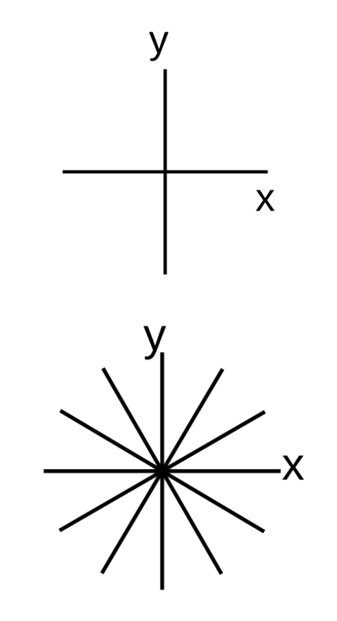
Model trend not only North-South and East-West, rotate coordinate axis by \(\alpha\)
(in figure: 30° and 60°)
20.4 Relative spatial distances as covariates
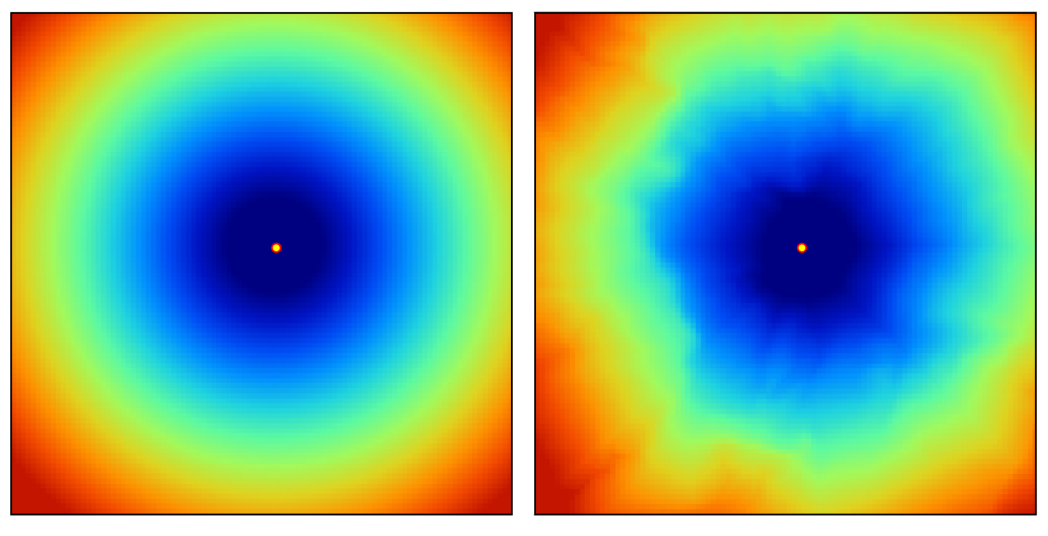
An additional set of covariates is defined based on the relative distance to each observation:
\[ X_G = \{d_{p_1}, d_{p_1}, ..., d_{p_n}\} \]
where \(d_{p_i}\) is the euclidean distance (or any other more complex proximity distance) to the observed location \(p_i\) and \(n\) is the total number of training observations.
For each \(n\) observations one covariate is added (R packages GSIF, spatialRF).
Example covariate layer for one observation by euclidean distance (left) or travel time distance (right).
20.5 Spatial neighbors as covariates
Include observed values from \(n\) nearest locations and distances to these locations.
For each \(n\) nearest neighbor 2 colums are added as covariates:
- value at \(n\)th nearest observation
- distance corresponding to the location contributing the observed value
\(n\) is a tuning parameter.
R package RFSI
20.6 Spatial random forest – summary
Currently no satisfactory solution.
Proposed methods are merely ad-hoc.
I suggest to keep it simple: Use roated coordiante axis.